Forest
Reference
3.13 Argument processor¶
For a gentle(r) introduction to the argument processor, see §2.6.
The argument processor takes a sequence of instructions and an arbitrary number of arguments and transforms the given arguments according to the instructions. This is the generic form of a process expression:
⟨process⟩ = ⟨instructions⟩⟨arg \(1\)⟩…⟨arg \(n\)⟩
There are three ways to invoke the argument processor: via handler .process, as one of the two alternatives of a ⟨forestmath⟩ expression and recursively, by its instruction P.
The result of the computation is passed on to the handled key as a sequence of arguments. When the argument processor is invoked this way, any number of items can be returned.1
⟨forestmath⟩ = ⟨pgfmath⟩ | >⟨process⟩
In words, a ⟨forestmath⟩ expression is either a ⟨pgfmath⟩ expression or an argument processor expression (⟨process⟩) prefixed by >.
In other words, Forest accepts an argument processor expression anywhere it accepts a ⟨pgfmath⟩ expression.2 To indicate that we’re providing an argument processor expression, we prefix it with >.
When the argument processor is invoked this way, it should return a single item.
The syntax of argument processor is a cross between expl3’s function argument specification and a Turing machine, spiced with a bit of reversed Polish notation. ;-)
Think of ⟨instructions⟩ as a program and ⟨arg \(1\)⟩…⟨arg \(n\)⟩ as the data that this program operates on.
If you’re familiar with Turing machines: like a Turing machine, the argument processor has a notion of a head; unlike a Turing machine, the argument processor head is positioned not over some argument, but between two arguments. If you’re not familiar with Turing machines: imagine the arguments as items on a tape and the argument processor as a head that is always located between some two items. As the head is between two arguments, we can talk about the arguments on the left and the arguments on the right.
In general, an instruction will take some items from the left and some from the right (deleting them from the tape), perform some computation and insert the result on the tape, some result items to the left and some to the right. However, most instructions simply take an item from the right, do something with it, and put the (single-item) result to the left; in effect, the head is moved one item to the right. At the beggining, all the arguments are always on the right, so the general idea is that the program will walk through the given arguments, processing them in order.
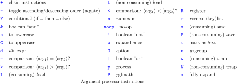
Descriptions of individual instructions, given below, contain (at the right edge of the page) the argument specification, which tells us about the number of input and output items and the movement of the head. The input and output are separated by an arrow (\(\longrightarrow\)), and the green eye (👁) signifies the position of the head with respect to the (input or output) items.
For example, instruction O, which converts an option name into the option value, exemplifies the most common scenario: it takes one argument from the right and puts the result to the left (in other words, the head moves one item to the right). Wrapping instrucion w is more complicated. Given instruction w\(n\), the argument processor takes one argument from the right (the wrapping macro body) and \(n\) items from the left (which become the arguments of the wrapping macro), and puts the resulting item to the left. Comparisons and boolean operations are the instructions resembling the reverse Polish notation: they take the arguments from the left and put the result to the left, as well. Finally, it is worth mentioning instructions noop and +, which simply move the head to the right and left, respectively; given that the usual movement of the head is to the right, + can be thought of as a process-the-argument-again instruction.
Before we finally list the available instructions, some notes:
⟨Instructions⟩ may be given in braces or not. If not, everything until the first opening brace is considered to be an instruction.
An argument item (⟨arg\(_k\)⟩) is a standard TeX macro argument: either a token or a braced token list. (The obvious exception: ⟨arg\(_1\)⟩ needs to be braced if it follows braceless instructions.)
Spaces in ⟨instructions⟩ and between arguments are ignored. Format your .process as you wish!
Instructions followed by [\(n\)] below take an optional numeric modifier.
The modifier should be given within the instruction string itself, immediately following the instruction. In particular, no spaces are allowed there. (Sorry for the little white lie above.) The number should not be enclosed in braces, even if it is more than one digit long.
This modifier is always optional: its default value varies from instruction to instruction. (Providing \(0\) means to use the default.)
Unless noted otherwise, the optional numerical argument \(n\) instruct the argument processor to repeat the previous instruction \(n\) times (by default, 1). For example, O3 is equivalent to OOO.
_[\(n\)] no-op 👁 ⟨arg⟩ → ⟨arg⟩ 👁 (processor)¶
The argument is not processed, but simply skipped over. In other words, this instruction only moves the head one item to the right. (This is like expl3’s argument specifier n.)
\(n\) means repetition.
When the end of the instructions is reached, any remaining arguments on the right are processed using this no-op instruction.
o[\(n\)] expand once 👁 ⟨arg⟩ → ⟨result⟩ 👁 (processor)¶
⟨arg⟩ is expanded once. (This is like expl3’s argument specifier o).
The operation is repeated \(n\) times (default, one) without moving the head between the repetition. For example, o3 expands the argument three times (and then moves the head right).
x fully expand 👁 ⟨arg⟩ → ⟨result⟩ 👁 (processor)¶
⟨arg⟩ is fully expanded using \edef. (This is like expl3’s argument specifier x.)
O[\(n\)] option 👁 ⟨option⟩ → ⟨result⟩ 👁 (processor)¶
⟨option⟩=\meta{option name}|\meta{relative node name}\texttt{.}\meta{option name}
In the former case, ⟨result⟩ is the value of option at the current node, in the latter, the value of option at the node referred to by ⟨relative node name⟩.
\(n\) means repetition.
R[\(n\)] register 👁 ⟨register⟩ → ⟨result⟩ 👁 (processor)¶
⟨result⟩ is the value of register ⟨register⟩.
\(n\) means repetition.
Execute an embedded call of the argument processor. The embedded argument processor may return any number of items.
\(n\) means repetition.
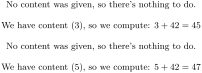
  \begin{forest}

    grow'=0, phantom,

    delay={for children={

      content/.process={_O= ? ~p~}

        {}{content}

        {_{No content was given, so there's nothing to do.}}

        {Ow1{content}{We have content (##1), so we compute:

                      $##1+42=\the\numexpr ##1+42$}}

      }}

    [[][3][][5]]

  \end{forest}
P[\(n\)] pgfmath 👁 ⟨pgfmath⟩ → ⟨result⟩ 👁 (processor)¶
⟨result⟩ is the result of evaluating ⟨pgfmath expr⟩ using \pgfmathparse.
\(n\) means repetition.
Combining P and w, .process is capable of anything .wrap \(n\) pgfmath args can do. Even better, as we can combine pgfmath and non-pgfmath methods, computations that use .process can be (much!) faster. Study the following examples to see how less and less pgfmath is used to achieve the same result — but note that such extreme antipgfmathism probably only makes sense for style/package developers in computations that get performed many times.

  \begin{forest}

    [,grow'=east, where level=1{}{phantom,ignore,ignore edge}

      [(a),delay={content/.wrap 4 pgfmath args={#1 $#2*#3=#4$}

           {content}{content("!1")}{content("!2")}{int(content("!1")*content("!2"))}}

        [6][7]]

      [(b),delay={content/.process={O OO~P~ w4}

        {content}

        {!1.content}{!2.content}{int(content("!1")*content("!2"))}

        {#1 $#2*#3=#4$}}

        [6][7]]

      [(c),delay={content/.process={O OO ~W2+P~ w4}

        {content}

        {!1.content}{!2.content}{int(#1*#2)}

        {#1 $#2*#3=#4$}}

        [6][7]]

      [(d),delay={content/.process={O OO ~W2+n~ w4}

        {content}

        {!1.content}{!2.content}{#1*#2}

        {#1 $#2*#3=#4$}}

        [6][7]]

    ]

  \end{forest}
n[\(n\)] numexpr 👁 ⟨numexpr⟩ → ⟨result⟩ 👁 (processor)¶
⟨result⟩ is the result of evaluating ⟨dimexpr⟩ using eTeX’s \number\numexpr.
\(n\) means repetition.
d[\(n\)] dimexpr 👁 ⟨dimexpr⟩ → ⟨result⟩ 👁 (processor)¶
⟨result⟩ is the result of evaluating ⟨dimexpr⟩ using eTeX’s \the\dimexpr.
\(n\) means repetition.
+[\(n\)] chain instructions ⟨arg⟩ 👁 → 👁 ⟨arg⟩(processor)¶
This action allows one to “process the same argument more than once”. It does not process the current argument (in fact, there need not be any current argument), but rather moves the last result back in the argument queue. In other words, our machine’s head moves one step left. You can also imagine it as an inverse of noop.
\(n\) means repetition.

  \begin{forest}

    test/.style n args={3}{align=center,

      content={The value of my option \texttt{#1} is \texttt{#2}.\\#3}}

    [~fit~,delay={test/.process={O ~O+O~}{content}~{content}~{Yes it is!}}]

  \end{forest}
w[\(n\)] (consuming) wrap ⟨arg\(_{1}\)⟩…⟨arg\(_{n}\)⟩ 👁 ⟨macro body⟩ → ⟨result⟩ 👁 (processor)¶
W[\(n\)] (non-consuming) wrap ⟨arg\(_{1}\)⟩…⟨arg\(_{n}\)⟩ 👁 ⟨macro body⟩ → ⟨arg\(_{1}\)⟩…⟨arg\(_{n}\)⟩⟨result⟩ 👁 (processor)¶
Defines a temporary macro with \(n\) undelimited arguments using the ⟨macro body⟩ given on the right and expands it (once). The arguments given to the temporary macro are taken from the left: ⟨arg\(_{1}\)⟩…⟨arg\(_{n}\)⟩. The result of the expansion is stored as ⟨result⟩ to the right.
With w, ⟨arg\(_{1}\)⟩…⟨arg\(_{n}\)⟩ are “consumed”, i.e. they are removed from the result list on the left. W keeps ⟨arg\(_{1}\)⟩…⟨arg\(_{n}\)⟩ in the result list.
Default \(n\) is 1. (Specifying \(n>9\) raises an error.)
&[\(n\)] boolean “and” * 👁 → 👁 (processor)¶
|[\(n\)] boolean “or” ⟨arg\(_{1}\)⟩⟨arg\(_{2}\)⟩ 👁 → ⟨result⟩ 👁 (processor)¶
⟨result⟩ is a boolean conjunction/disjunction of \(n\) arguments. The arguments are taken from the left. They should be numbers (positive integers): 0 means false, any other number means true. The ⟨result⟩ is always 0 or 1.
Default \(n\) is 2.
! boolean “not” ⟨arg⟩ 👁 → ⟨result⟩ 👁 (processor)¶
⟨result⟩ is a boolean negation of the argument. The argument is taken from the left. It should be a number (positive integer): 0 means false, any other number means true. The ⟨result⟩ is always 0 or 1.
? conditional (if … then … else) ⟨condition⟩ 👁 ⟨true arg⟩⟨false arg⟩ → 👁 ⟨result⟩(processor)¶
⟨result⟩ is ⟨true arg⟩ is ⟨condition⟩ is true (non-zero), otherwise ⟨false arg⟩.
The condition is taken from the left. The true and false arguments are expected on the right, where the winner is left as well.
= comparison: \(\protect\meta{arg\)_1\(}=\protect\meta{arg\)_2\(}\)? * 👁 → 👁 (processor)¶
< comparison: \(\protect\meta{arg\)_1\(}<\protect\meta{arg\)_2\(}\)? * 👁 → 👁 (processor)¶
> comparison: \(\protect\meta{arg\)_1\(}\protect\greaterthan\protect\meta{arg\)_2\(}\)? ⟨arg\(_{1}\)⟩⟨arg\(_{2}\)⟩ 👁 → ⟨result⟩ 👁 (processor)¶
Compare ⟨arg\(_{1}\)⟩ and ⟨arg\(_{2}\)⟩, returning 1 (true) if ⟨arg\(_{1}\)⟩ is equal to / less than / greater than ⟨arg\(_{2}\)⟩, 0 (false) otherwise.
The arguments are taken from the left. They can be either numbers, dimensions, text or token lists. Both arguments are expected to be of the same type. The type of comparison is determined by the type of the result returned by the last instruction. O/R look up the type of option/register to determine the type (booleans are numbers and keylists are toks). Text type must be marked explicitely using t.
Comparison is carried out using \ifnum for numbers, \ifdim for dimensions (this includes unitless decimals returned by pgfmath) and \pdfstrcmp3 for text — for these three types, all three comparison operators are supported. For generic token lists, only = makes sense and is carried out using \ifx.
In the following example, (a) performs lexicographical comparison because we have marked 21 as text; (b) and (c) perform numeric comparison: in (b), the type is automatically determined from the type of register tempcounta, in (c) 21 is marked manually using n.

  \forestset{

    tempcounta=100,

    TeX/.process={Rw1}{tempcounta}{$#1>21$?\ },

    TeX={(a)\ }, if={>{Rt>}{tempcounta}{21}}{TeX=yes}{TeX=no},TeX={,\ },

    TeX={(b)\ }, if={>{_R<}{21}{tempcounta}}{TeX=yes}{TeX=no},TeX={,\ },

    TeX={(c)\ }, if={>{Rn>}{tempcounta}{21}}{TeX=yes}{TeX=no},

  }
c to lowercase 👁 ⟨arg⟩ → ⟨result⟩ 👁 (processor)¶
C to uppercase 👁 ⟨arg⟩ → ⟨result⟩ 👁 (processor)¶
- toggle ascending/descending order (negate) ⟨arg⟩ 👁 → ⟨result⟩ 👁 (processor)¶
If the argument is of the text type, its sorting order is changed from ascending to descending or vice versa.
For any numerical argument type (number, dimension, unitless dimension), the argument is actually negated, which obviously has the same effect on sorting.
For generic type arguments, this operation is a no-op.
u ungroup 👁 ⟨arg⟩ → 👁 ⟨item\(_1\)⟩…⟨item\(_n\)⟩(processor)¶
As every TeX undelimited macro argument, ⟨arg⟩ is a list of tokens or braced token lists. This instruction puts those items back to the right as “separate arguments”.
s[\(n\)] (consuming) save ⟨arg\(_{1}\)⟩…⟨arg\(_{n}\)⟩ 👁 → 👁 (processor)¶
S[\(n\)] (non-consuming) save ⟨arg\(_{1}\)⟩…⟨arg\(_{n}\)⟩ 👁 → ⟨arg\(_{1}\)⟩…⟨arg\(_{n}\)⟩ 👁 (processor)¶
Saves the last \(n\) arguments from the left into a “special place”.
With s, ⟨arg\(_{1}\)⟩…⟨arg\(_{n}\)⟩ are “consumed”, i.e. they are removed from the result list on the left. S keeps ⟨arg\(_{1}\)⟩…⟨arg\(_{n}\)⟩ in the result list.
Default \(n\) is 1.
l[\(n\)] (consuming) load 👁 → ⟨arg\(_{1}\)⟩…⟨arg\(_{n}\)⟩ 👁 (processor)¶
L[\(n\)] (non-consuming) load 👁 → ⟨arg\(_{1}\)⟩…⟨arg\(_{n}\)⟩ 👁 (processor)¶
Loads last \(n\) arguments from the “special place” to the left.
With l, ⟨arg\(_{1}\)⟩…⟨arg\(_{n}\)⟩ are “consumed”, i.e. they are removed from the special place. S keeps ⟨arg\(_{1}\)⟩…⟨arg\(_{n}\)⟩ in the special place.
The default \(n\) is 0 and indicates that the entire special place should be loaded.
r reverse (key)list 👁 ⟨list⟩ → ⟨result⟩ 👁 (processor)¶
⟨list⟩ should be a comma-separated list (not a name of a keylist option or register). ⟨result⟩ contains the same elements in the reverse order.