TikZ and PGF Manual
TikZ
25 Transformations
pgf has a powerful transformation mechanism that is similar to the transformation capabilities of metafont. The present section explains how you can access it in TikZ.
25.1 The Different Coordinate Systems
It is a long process from a coordinate like, say, \((1,2)\) or \((1\mathrm {cm},5\mathrm {pt})\), to the position a point is finally placed on the display or paper. In order to find out where the point should go, it is constantly “transformed”, which means that it is mostly shifted around and possibly rotated, slanted, scaled, and otherwise mutilated.
In detail, (at least) the following transformations are applied to a coordinate like \((1,2)\) before a point on the screen is chosen:
-
1. pgf interprets a coordinate like \((1,2)\) in its \(xy\)-coordinate system as “add the current \(x\)-vector once and the current \(y\)-vector twice to obtain the new point”.
-
2. pgf applies its coordinate transformation matrix to the resulting coordinate. This yields the final position of the point inside the picture.
-
3. The backend driver (like dvips or pdftex) adds transformation commands such that the coordinate is shifted to the correct position in TeX’s page coordinate system.
-
4. pdf (or PostScript) apply the canvas transformation matrix to the point, which can once more change the position on the page.
-
5. The viewer application or the printer applies the device transformation matrix to transform the coordinate to its final pixel coordinate on the screen or paper.
In reality, the process is even more involved, but the above should give the idea: A point is constantly transformed by changes of the coordinate system.
In TikZ, you only have access to the first two coordinate systems: The \(xy\)-coordinate system and the coordinate transformation matrix (these will be explained later). pgf also allows you to change the canvas transformation matrix, but you have to use commands of the core layer directly to do so and you “better know what you are doing” when you do this. The moment you start modifying the canvas matrix, pgf immediately loses track of all coordinates and shapes, anchors, and bounding box computations will no longer work.
25.2 The XY- and XYZ-Coordinate Systems
The first and easiest coordinate systems are pgf’s \(xy\)- and \(xyz\)-coordinate systems. The idea is very simple: Whenever you specify a coordinate like (2,3) this means \(2v_x + 3v_y\), where \(v_x\) is the current \(x\)-vector and \(v_y\) is the current \(y\)-vector. Similarly, the coordinate (1,2,3) means \(v_x + 2v_y + 3v_z\).
Unlike other packages, pgf does not insist that \(v_x\) actually has a \(y\)-component of \(0\), that is, that it is a horizontal vector. Instead, the \(x\)-vector can point anywhere you want. Naturally, normally you will want the \(x\)-vector to point horizontally.
One undesirable effect of this flexibility is that it is not possible to provide mixed coordinates as in \((1,2\mathrm {pt})\). Life is hard.
To change the \(x\)-, \(y\)-, and \(z\)-vectors, you can use the following options:
-
/tikz/x=⟨value⟩ (no default, initially 1cm) 
If ⟨value⟩ is a dimension, the \(x\)-vector of pgf’s \(xyz\)-coordinate system is set up to point ⟨value⟩ to the right, that is, to (⟨value⟩,0pt).
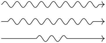
                    \begin{tikzpicture}

                      \draw                  (0,0)   --
                    +(1,0);

                      \draw[x=2cm,color=red] (0,0.1) --
                    +(1,0);

                    \end{tikzpicture}

The last example shows that the size of steppings in grids, just like all other dimensions, are not affected by the \(x\)-vector. After all, the \(x\)-vector is only used to determine the coordinate of the upper right corner of the grid.
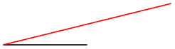
If ⟨value⟩ is a coordinate, the \(x\)-vector of pgf’s \(xyz\)-coordinate system is set to the specified coordinate. If ⟨value⟩ contains a comma, it must be put in braces.
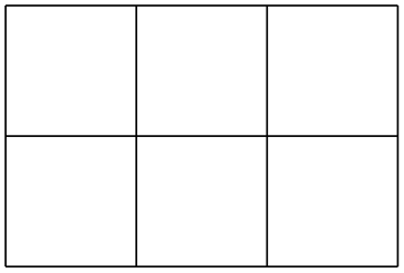
                    \begin{tikzpicture}

                      \draw                            (0,0) --
                    (1,0);

                      \draw[x={(2cm,0.5cm)},color=red] (0,0) --
                    (1,0);

                    \end{tikzpicture}
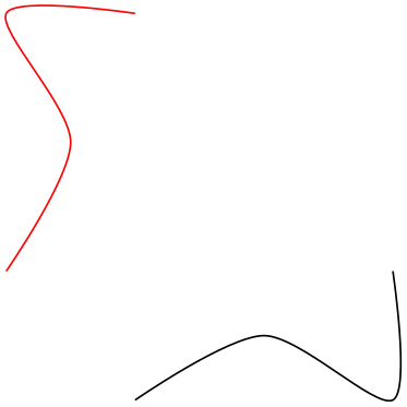
You can use this, for example, to exchange the meaning of the \(x\)- and \(y\)-coordinate.
                    \begin{tikzpicture}[smooth]

                      \draw plot
                    coordinates{(1,0) (2,0.5) (3,0) (3,1)};

                      \draw[x={(0cm,1cm)},y={(1cm,0cm)},color=red]

                            plot
                    coordinates{(1,0) (2,0.5) (3,0) (3,1)};

                    \end{tikzpicture}
-
/tikz/y=⟨value⟩ (no default, initially 1cm) 
Works like the x= option, only if ⟨value⟩ is a dimension, the resulting vector points to (0,⟨value⟩).
-
/tikz/z=⟨value⟩ (no default, initially \(-3.85\)mm) 
Works like the y= option, but now a dimension is the point (⟨value⟩,⟨value⟩).
25.3 Coordinate Transformations
pgf and TikZ allow you to specify coordinate transformations. Whenever you specify a coordinate as in (1,0) or (1cm,1pt) or (30:2cm), this coordinate is first “reduced” to a position of the form “\(x\) points to the right and \(y\) points upwards”. For example, (1in,5pt) is reduced to “\(72\frac {27}{100}\) points to the right and 5 points upwards” and (90:100pt) means “0pt to the right and 100 points upwards”.
The next step is to apply the current coordinate transformation matrix to the coordinate. For example, the coordinate transformation matrix might currently be set such that it adds a certain constant to the \(x\) value. Also, it might be set up such that it, say, exchanges the \(x\) and \(y\) value. In general, any “standard” transformation like translation, rotation, slanting, or scaling or any combination thereof is possible. (Internally, pgf keeps track of a coordinate transformation matrix very much like the concatenation matrix used by pdf or PostScript.)
The most important aspect of the coordinate transformation matrix is that it applies to coordinates only! In particular, the coordinate transformation has no effect on things like the line width or the dash pattern or the shading angle. In certain cases, it is not immediately clear whether the coordinate transformation matrix should apply to a certain dimension. For example, should the coordinate transformation matrix apply to grids? (It does.) And what about the size of arced corners? (It does not.) The general rule is: “If there is no ‘coordinate’ involved, even ‘indirectly’, the matrix is not applied.”. However, sometimes, you simply have to try or look it up in the documentation whether the matrix will be applied.
Setting the matrix cannot be done directly. Rather, all you can do is to “add” another transformation to the current matrix. However, all transformations are local to the current TeX-group. All transformations are added using graphic options, which are described below.
Transformations apply immediately when they are encountered “in the middle of a path” and they apply only to the coordinates on the path following the transformation option.
A final word of warning: You should refrain from using “aggressive” transformations like a scaling of a factor of 10 000. The reason is that all transformations are done using TeX, which has a fairly low accuracy. Furthermore, in certain situations it is necessary that TikZ inverts the current transformation matrix and this will fail if the transformation matrix is badly conditioned or even singular (if you do not know what singular matrices are, you are blessed).
-
/tikz/shift={⟨coordinate⟩}(no default) 
Adds the ⟨coordinate⟩ to all coordinates.

-
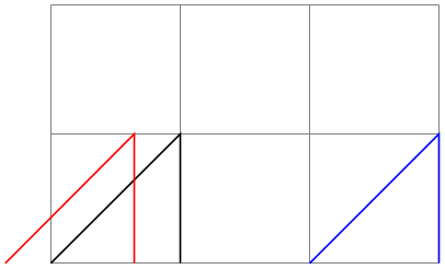
/tikz/shift only(no value) 
This option does not take any parameter. Its effect is to cancel all current transformations except for the shifting. This means that the origin will remain where it is, but any rotation around the origin or scaling relative to the origin or skewing will no longer have an effect.
This option is useful in situations where a complicated transformation is used to “get to a position”, but you then wish to draw something “normal” at this position.
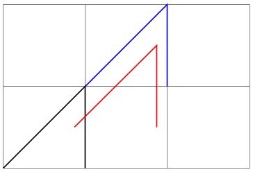
                    \begin{tikzpicture}

                      \draw[help lines] (0,0) grid
                    (3,2);

                      \draw                                      (0,0) --
                    (1,1) --
                    (1,0);

                      \draw[rotate=30,xshift=2cm,blue]           (0,0) --
                    (1,1) --
                    (1,0);

                      \draw[rotate=30,xshift=2cm,shift only,red] (0,0) --
                    (1,1) --
                    (1,0);

                    \end{tikzpicture}
-
/tikz/xshift=⟨dimension⟩(no default) 
Adds ⟨dimension⟩ to the \(x\) value of all coordinates.
-
/tikz/yshift=⟨dimension⟩(no default) 
Adds ⟨dimension⟩ to the \(y\) value of all coordinates.
-
/tikz/scale=⟨factor⟩(no default) 
Multiplies all coordinates by the given ⟨factor⟩. The ⟨factor⟩ should not be excessively large in absolute terms or very close to zero.
-
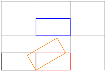
/tikz/scale around={⟨factor⟩:⟨coordinate⟩}(no default) 
Scales the coordinate system by ⟨factor⟩, with the “origin of scaling” centered on ⟨coordinate⟩ rather than the origin.
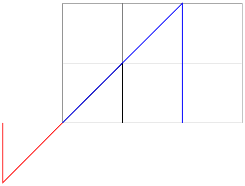
                    \begin{tikzpicture}

                      \draw[help lines] (0,0) grid
                    (3,2);

                      \draw                             (0,0) --
                    (1,1) --
                    (1,0);

                      \draw[scale=2,blue]               (0,0) --
                    (1,1) --
                    (1,0);

                      \draw[scale around={2:(1,1)},red] (0,0) --
                    (1,1) --
                    (1,0);

                    \end{tikzpicture}
-
/tikz/xscale=⟨factor⟩(no default) 
Multiplies only the \(x\)-value of all coordinates by the given ⟨factor⟩.
-
/tikz/yscale=⟨factor⟩(no default) 
Multiplies only the \(y\)-value of all coordinates by ⟨factor⟩.
-
/tikz/xslant=⟨factor⟩(no default) 
Slants the coordinate horizontally by the given ⟨factor⟩:
-
/tikz/yslant=⟨factor⟩(no default) 
Slants the coordinate vertically by the given ⟨factor⟩:
-
/tikz/rotate=⟨degree⟩(no default) 
Rotates the coordinate system by ⟨degree⟩:

-
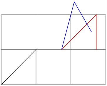
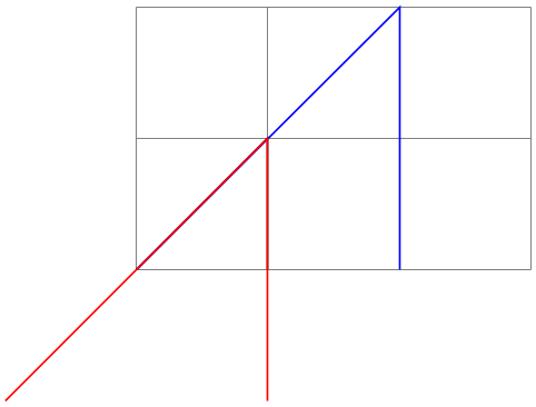
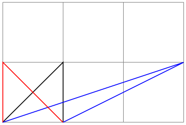
/tikz/rotate around={⟨degree⟩:⟨coordinate⟩}(no default) 
Rotates the coordinate system by ⟨degree⟩ around the point ⟨coordinate⟩.

                    \begin{tikzpicture}

                      \draw[help lines] (0,0) grid
                    (3,2);

                      \draw                                (0,0) --
                    (1,1) --
                    (1,0);

                      \draw[rotate around={40:(1,1)},blue] (0,0) --
                    (1,1) --
                    (1,0);

                      \draw[rotate around={-20:(1,1)},red] (0,0) --
                    (1,1) --
                    (1,0);

                    \end{tikzpicture}
-
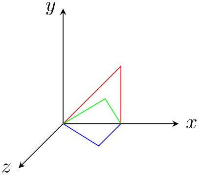
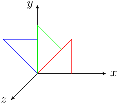
/tikz/rotate around x=⟨angle⟩(no default) 
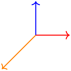
This key sets the \(x\), \(y\) and \(z\) vectors of the pgf \(xyz\)-coordinate system so that they are rotated by ⟨angle⟩ around the axis corresponding to the \(x\)-vector. The rotation is applied so that when looking towards the origin along this axis, positive angles result in an anticlockwise rotation.
                    \begin{tikzpicture}[>=stealth]

                      \draw [->] (0,0,0) --
                    (2,0,0) node
                    [at end, right] {$x$};

                      \draw [->] (0,0,0) --
                    (0,2,0) node
                    [at end, left]  {$y$};

                      \draw [->] (0,0,0) --
                    (0,0,2) node
                    [at end, left]  {$z$};


                      \draw [red,   rotate around x=0]  (0,0,0) --
                    (1,1,0) --
                    (1,0,0);

                      \draw [green, rotate around x=45] (0,0,0) --
                    (1,1,0) --
                    (1,0,0);

                      \draw [blue,  rotate around x=90] (0,0,0) --
                    (1,1,0) --
                    (1,0,0);

                    \end{tikzpicture}
-
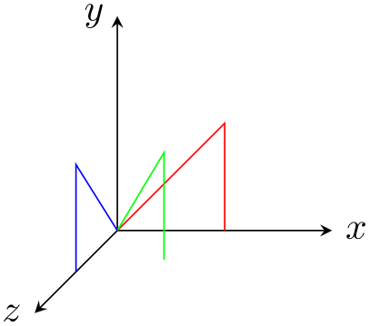
/tikz/rotate around y=⟨angle⟩(no default) 
This key sets the \(x\), \(y\) and \(z\) vectors of the pgf \(xyz\)-coordinate system so that they are rotated by ⟨angle⟩ around the axis corresponding to the \(y\)-vector. The rotation is applied so that when looking towards the origin along this axis, positive angles result in an anticlockwise rotation.
                    \begin{tikzpicture}[>=stealth]

                      \draw [->] (0,0,0) --
                    (2,0,0) node
                    [at end, right] {$x$};

                      \draw [->] (0,0,0) --
                    (0,2,0) node
                    [at end, left]  {$y$};

                      \draw [->] (0,0,0) --
                    (0,0,2) node
                    [at end, left]  {$z$};


                      \draw [red,   rotate around y=0]   (0,0,0) --
                    (1,1,0) --
                    (1,0,0);

                      \draw [green, rotate around y=-45] (0,0,0) --
                    (1,1,0) --
                    (1,0,0);

                      \draw [blue,  rotate around y=-90] (0,0,0) --
                    (1,1,0) --
                    (1,0,0);

                    \end{tikzpicture}
-
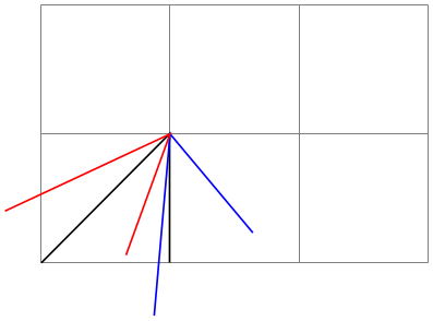
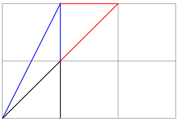
/tikz/rotate around z=⟨angle⟩(no default) 
This key sets the \(x\), \(y\) and \(z\) vectors of the pgf \(xyz\)-coordinate system so that they are rotated by ⟨angle⟩ around the axis corresponding to the \(z\)-vector. The rotation is applied so that when looking towards the origin along this axis, positive angles result in an anticlockwise rotation.
                    \begin{tikzpicture}[>=stealth]

                      \draw [->] (0,0,0) --
                    (2,0,0) node
                    [at end, right] {$x$};

                      \draw [->] (0,0,0) --
                    (0,2,0) node
                    [at end, left]  {$y$};

                      \draw [->] (0,0,0) --
                    (0,0,2) node
                    [at end, left]  {$z$};


                      \draw [red,   rotate around z=0]  (0,0) --
                    (1,1) --
                    (1,0);

                      \draw [green, rotate around z=45] (0,0) --
                    (1,1) --
                    (1,0);

                      \draw [blue,  rotate around z=90] (0,0) --
                    (1,1) --
                    (1,0);

                    \end{tikzpicture}
-
/tikz/cm={⟨\(a\)⟩,⟨\(b\)⟩,⟨\(c\)⟩,⟨\(d\)⟩,⟨coordinate⟩}(no default) 
applies the following transformation to all coordinates: Let \((x,y)\) be the coordinate to be transformed and let ⟨coordinate⟩ specify the point \((t_x,t_y)\). Then the new coordinate is given by \(\left (\begin {smallmatrix} a & c \\ b & d\end {smallmatrix}\right ) \left (\begin {smallmatrix} x \\ y \end {smallmatrix}\right ) + \left (\begin {smallmatrix} t_x \\ t_y \end {smallmatrix}\right )\). Usually, you do not use this option directly.
-
/tikz/reset cm(no value) 
Completely resets the coordinate transformation matrix to the identity matrix. This will destroy not only the transformations applied in the current scope, but also all transformations inherited from surrounding scopes. Do not use this option, unless you really, really know what you are doing.
25.4 Canvas Transformations
A canvas transformation, see Section 99.4 for details, is best thought of as a transformation in which the drawing canvas is stretched or rotated. Imaging writing something on a balloon (the canvas) and then blowing air into the balloon: Not only does the text become larger, the thin lines also become larger. In particular, if you scale the canvas by a factor of two, all lines are twice as thick.
Canvas transformations should be used with great care. In most circumstances you do not want line widths to change in a picture as this creates visual inconsistency.
Just as important, when you use canvas transformations pgf loses track of positions of nodes and of picture sizes since it does not take the effect of canvas transformations into account when it computes coordinates of nodes (do not, however, rely on this; it may change in the future).
Finally, note that a canvas transformation always applies to a path as a whole, it is not possible (as for coordinate transformations) to use different transformations in different parts of a path.
In short, you should not use canvas transformations unless you really know what you are doing.
-
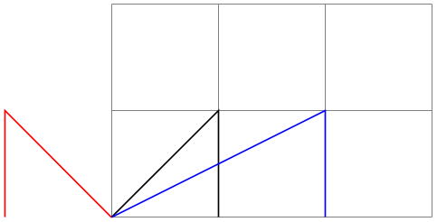
/tikz/transform canvas=⟨options⟩(no default) 
The ⟨options⟩ should contain coordinate transformations options like scale or xshift. Multiple options can be given, their effects accumulate in the usual manner. The effect of these ⟨options⟩ (immediately) changes the current canvas transformation matrix. The coordinate transformation matrix is not changed. Tracking of the picture size is (locally) switched off and the node coordinate will no longer be correct.
                    \begin{tikzpicture}

                      \draw[help lines] (0,0) grid
                    (3,2);

                      \draw                                    (0,0) --
                    (1,1) --
                    (1,0);

                      \draw[transform canvas={scale=2},blue]   (0,0) --
                    (1,1) --
                    (1,0);

                      \draw[transform canvas={rotate=180},red] (0,0) --
                    (1,1) --
                    (1,0);

                    \end{tikzpicture}