TikZ and PGF Manual
Tutorials and Guidelines
4 Tutorial: Euclid’s Amber Version of the Elements
In this third tutorial we have a look at how TikZ can be used to draw geometric constructions.
Euclid is currently quite busy writing his new book series, whose working title is “Elements” (Euclid is not quite sure whether this title will convey the message of the series to future generations correctly, but he intends to change the title before it goes to the publisher). Up to now, he wrote down his text and graphics on papyrus, but his publisher suddenly insists that he must submit in electronic form. Euclid tries to argue with the publisher that electronics will only be discovered thousands of years later, but the publisher informs him that the use of papyrus is no longer cutting edge technology and Euclid will just have to keep up with modern tools.
Slightly disgruntled, Euclid starts converting his papyrus entitled “Book I, Proposition I” to an amber version.
4.1 Book I, Proposition I
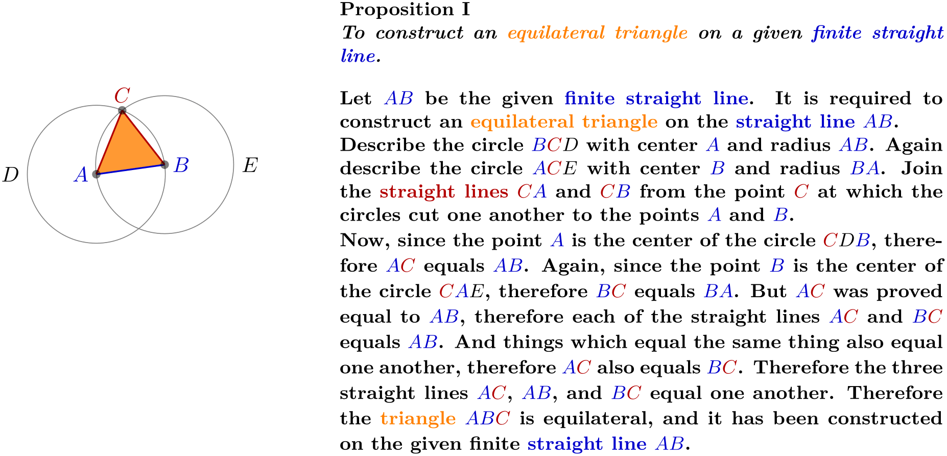
The drawing on his papyrus looks like this:1
Let us have a look at how Euclid can turn this into TikZ code.
1 The text is taken from the wonderful interactive version of Euclid’s Elements by David E. Joyce, to be found on his website at Clark University.
4.1.1 Setting up the Environment
As in the previous tutorials, Euclid needs to load TikZ, together with some libraries. These libraries are calc, intersections, through, and backgrounds. Depending on which format he uses, Euclid would use one of the following in the preamble:
                % For LaTeX:

                \usepackage{tikz}

                \usetikzlibrary{calc,intersections,through,backgrounds}
                % For plain TeX:

                \input tikz.tex

                \usetikzlibrary{calc,intersections,through,backgrounds}
                % For ConTeXt:

                \usemodule[tikz]

                \usetikzlibrary[calc,intersections,through,backgrounds]
4.1.2 The Line AB
The first part of the picture that Euclid wishes to draw is the line \(AB\). That is easy enough, something like \draw (0,0) -- (2,1); might do. However, Euclid does not wish to reference the two points \(A\) and \(B\) as \((0,0)\) and \((2,1)\) subsequently. Rather, he wishes to just write A and B. Indeed, the whole point of his book is that the points \(A\) and \(B\) can be arbitrary and all other points (like \(C\)) are constructed in terms of their positions. It would not do if Euclid were to write down the coordinates of \(C\) explicitly.
So, Euclid starts with defining two coordinates using the \coordinate command:

                \begin{tikzpicture}

                  \coordinate (A) at
                (0,0);

                  \coordinate (B) at
                (1.25,0.25);


                  \draw[blue] (A) --
                (B);

                \end{tikzpicture}
That was easy enough. What is missing at this point are the labels for the coordinates. Euclid does not want them on the points, but next to them. He decides to use the label option:

                \begin{tikzpicture}

                  \coordinate [label=left:\textcolor{blue}{$A$}]  (A) at
                (0,0);

                  \coordinate [label=right:\textcolor{blue}{$B$}] (B) at
                (1.25,0.25);


                  \draw[blue] (A) --
                (B);

                \end{tikzpicture}
At this point, Euclid decides that it would be even nicer if the points \(A\) and \(B\) were in some sense “random”. Then, neither Euclid nor the reader can make the mistake of taking “anything for granted” concerning these position of these points. Euclid is pleased to learn that there is a rand function in TikZ that does exactly what he needs: It produces a number between \(-1\) and \(1\). Since TikZ can do a bit of math, Euclid can change the coordinates of the points as follows:
                \coordinate [...] (A) at
                (0+0.1*rand,0+0.1*rand);

                \coordinate [...] (B) at
                (1.25+0.1*rand,0.25+0.1*rand);
This works fine. However, Euclid is not quite satisfied since he would prefer that the “main coordinates” \((0,0)\) and \((1.25,0.25)\) are “kept separate” from the perturbation \(0.1(\mathit {rand},\mathit {rand})\). This means, he would like to specify that coordinate \(A\) as “the point that is at \((0,0)\) plus one tenth of the vector \((\mathit {rand},\mathit {rand})\)”.
It turns out that the calc library allows him to do exactly this kind of computation. When this library is loaded, you can use special coordinates that start with ($ and end with $) rather than just ( and ). Inside these special coordinates you can give a linear combination of coordinates. (Note that the dollar signs are only intended to signal that a “computation” is going on; no mathematical typesetting is done.)
The new code for the coordinates is the following:
                \coordinate [...] (A) at
                ($ (0,0) +
                .1*(rand,rand) $);

                \coordinate [...] (B) at
                ($ (1.25,0.25) +
                .1*(rand,rand) $);
Note that if a coordinate in such a computation has a factor (like .1), you must place a * directly before the opening parenthesis of the coordinate. You can nest such computations.
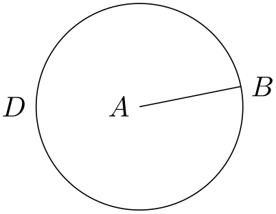
4.1.3 The Circle Around A
The first tricky construction is the circle around \(A\). We will see later how to do this in a very simple manner, but first let us do it the “hard” way.
The idea is the following: We draw a circle around the point \(A\) whose radius is given by the length of the line \(AB\). The difficulty lies in computing the length of this line.
Two ideas “nearly” solve this problem: First, we can write ($ (A) - (B) $) for the vector that is the difference between \(A\) and \(B\). All we need is the length of this vector. Second, given two numbers \(x\) and \(y\), one can write veclen(\(x\),\(y\)) inside a mathematical expression. This gives the value \(\sqrt {x^2+y^2}\), which is exactly the desired length.
The only remaining problem is to access the \(x\)- and \(y\)-coordinate of the vector \(AB\). For this, we need a new concept: the let operation. A let operation can be given anywhere on a path where a normal path operation like a line-to or a move-to is expected. The effect of a let operation is to evaluate some coordinates and to assign the results to special macros. These macros make it easy to access the \(x\)- and \(y\)-coordinates of the coordinates.
Euclid would write the following:
                \usetikzlibrary {calc}

                \begin{tikzpicture}

                  \coordinate [label=left:$A$]  (A) at
                (0,0);

                  \coordinate [label=right:$B$] (B) at
                (1.25,0.25);

                  \draw (A) --
                (B);


                  \draw (A) let

                              \p1 =
                ($ (B) -
                (A) $)

                            in

                              circle
                ({veclen(\x1,\y1)});

                \end{tikzpicture}
Each assignment in a let operation starts with \p, usually followed by a ⟨digit⟩. Then comes an equal sign and a coordinate. The coordinate is evaluated and the result is stored internally. From then on you can use the following expressions:
-
1. \x⟨digit⟩ yields the \(x\)-coordinate of the resulting point.
-
2. \y⟨digit⟩ yields the \(y\)-coordinate of the resulting point.
-
3. \p⟨digit⟩ yields the same as \x⟨digit⟩,\y⟨digit⟩.
You can have multiple assignments in a let operation, just separate them with commas. In later assignments you can already use the results of earlier assignments.
Note that \p1 is not a coordinate in the usual sense. Rather, it just expands to a string like 10pt,20pt. So, you cannot write, for instance, (\p1.center) since this would just expand to (10pt,20pt.center), which makes no sense.
Next, we want to draw both circles at the same time. Each time the radius is veclen(\x1,\y1). It seems natural to compute this radius only once. For this, we can also use a let operation: Instead of writing \p1 = ..., we write \n2 = .... Here, “n” stands for “number” (while “p” stands for “point”). The assignment of a number should be followed by a number in curly braces.
                \usetikzlibrary {calc}

                \begin{tikzpicture}

                  \coordinate [label=left:$A$]  (A) at
                (0,0);

                  \coordinate [label=right:$B$] (B) at
                (1.25,0.25);

                  \draw (A) --
                (B);


                  \draw let
                \p1 =
                ($ (B) -
                (A) $),

                            \n2 = {veclen(\x1,\y1)}

                        in

                          (A) circle
                (\n2)

                          (B) circle
                (\n2);

                \end{tikzpicture}
In the above example, you may wonder, what \n1 would yield? The answer is that it would be undefined – the \p, \x, and \y macros refer to the same logical point, while the \n macro has “its own namespace”. We could even have replaced \n2 in the example by \n1 and it would still work. Indeed, the digits following these macros are just normal TeX parameters. We could also use a longer name, but then we have to use curly braces:

                \usetikzlibrary {calc}

                \begin{tikzpicture}

                  \coordinate [label=left:$A$]  (A) at
                (0,0);

                  \coordinate [label=right:$B$] (B) at
                (1.25,0.25);

                  \draw (A) --
                (B);


                  \draw let
                \p1        =
                ($ (B) -
                (A) $),

                            \n{radius} = {veclen(\x1,\y1)}

                        in

                          (A) circle
                (\n{radius})

                          (B) circle
                (\n{radius});

                \end{tikzpicture}
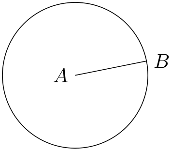
At the beginning of this section it was promised that there is an easier way to create the desired circle. The trick is to use the through library. As the name suggests, it contains code for creating shapes that go through a given point.
The option that we are looking for is circle through. This option is given to a node and has the following effects: First, it causes the node’s inner and outer separations to be set to zero. Then it sets the shape of the node to circle. Finally, it sets the radius of the node such that it goes through the parameter given to circle through. This radius is computed in essentially the same way as above.
                \usetikzlibrary {through}

                \begin{tikzpicture}

                  \coordinate [label=left:$A$]  (A) at
                (0,0);

                  \coordinate [label=right:$B$] (B) at
                (1.25,0.25);

                  \draw (A) --
                (B);


                  \node [draw,circle through=(B),label=left:$D$] at
                (A) {};

                \end{tikzpicture}
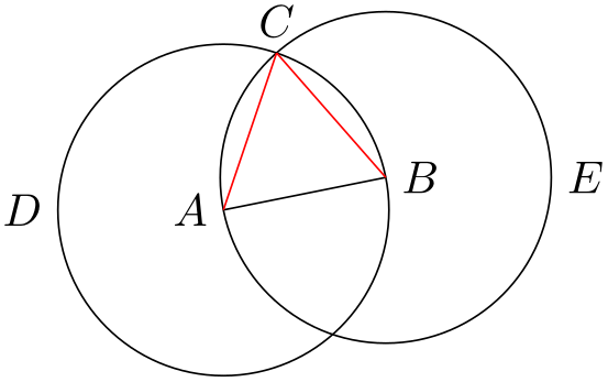
4.1.4 The Intersection of the Circles
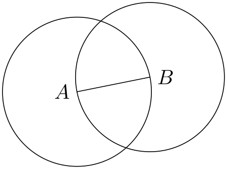
Euclid can now draw the line and the circles. The final problem is to compute the intersection of the two circles. This computation is a bit involved if you want to do it “by hand”. Fortunately, the intersections library allows us to compute the intersection of arbitrary paths.
The idea is simple: First, you “name” two paths using the name path option. Then, at some later point, you can use the option name intersections, which creates coordinates called intersection-1, intersection-2, and so on at all intersections of the paths. Euclid assigns the names D and E to the paths of the two circles (which happen to be the same names as the nodes themselves, but nodes and their paths live in different “namespaces”).
                \usetikzlibrary {intersections,through}

                \begin{tikzpicture}

                  \coordinate [label=left:$A$]  (A) at
                (0,0);

                  \coordinate [label=right:$B$] (B) at
                (1.25,0.25);

                  \draw (A) --
                (B);


                  \node (D) [name path=D,draw,circle through=(B),label=left:$D$]  at
                (A) {};

                  \node (E) [name path=E,draw,circle through=(A),label=right:$E$] at
                (B) {};


                  % Name the coordinates, but do not draw anything:

                  \path [name intersections={of=D and E}];


                  \coordinate [label=above:$C$] (C) at
                (intersection-1);


                  \draw [red] (A) --
                (C);

                  \draw [red] (B) --
                (C);

                \end{tikzpicture}
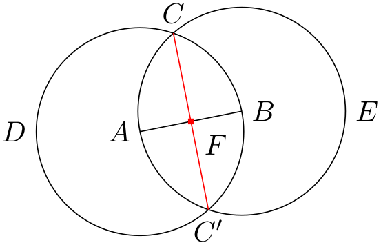
It turns out that this can be further shortened: The name intersections takes an optional argument by, which lets you specify names for the coordinates and options for them. This creates more compact code. Although Euclid does not need it for the current picture, it is just a small step to computing the bisection of the line \(AB\):
                \usetikzlibrary {intersections,through}

                \begin{tikzpicture}

                  \coordinate [label=left:$A$]  (A) at
                (0,0);

                  \coordinate [label=right:$B$] (B) at
                (1.25,0.25);

                  \draw [name path=A--B] (A) --
                (B);


                  \node (D) [name path=D,draw,circle through=(B),label=left:$D$]  at
                (A) {};

                  \node (E) [name path=E,draw,circle through=(A),label=right:$E$] at
                (B) {};


                  \path [name intersections={of=D and E, by={[label=above:$C$]C, [label=below:$C'$]C'}}];


                  \draw [name path=C--C',red] (C) --
                (C');


                  \path [name intersections={of=A--B and C--C',by=F}];

                  \node [fill=red,inner sep=1pt,label=-45:$F$] at
                (F) {};

                \end{tikzpicture}
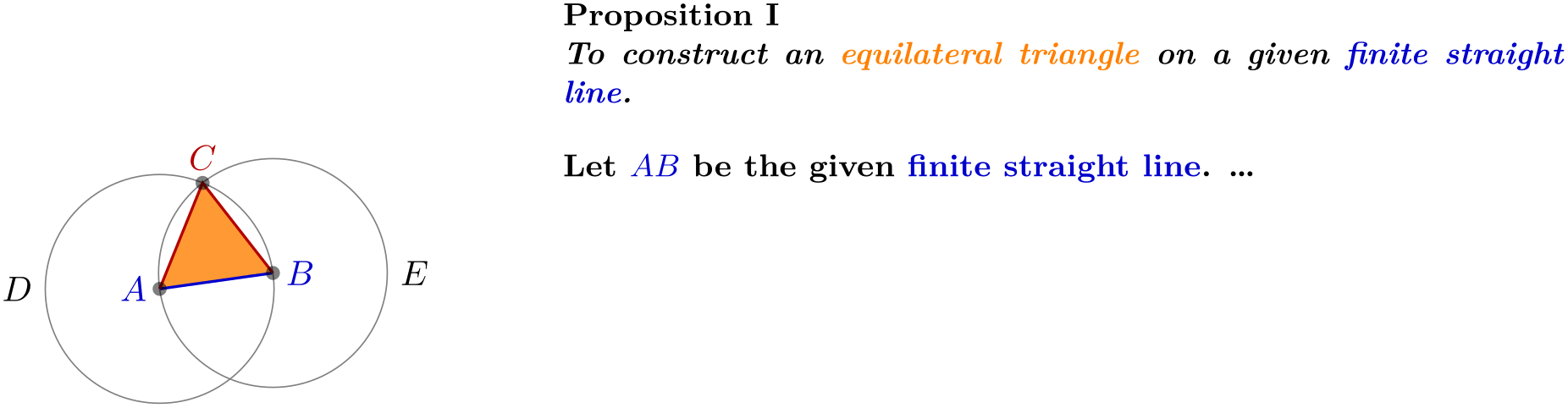
4.1.5 The Complete Code
Back to Euclid’s code. He introduces a few macros to make life simpler, like a \A macro for typesetting a blue \(A\). He also uses the background layer for drawing the triangle behind everything at the end.
                \usetikzlibrary {backgrounds,calc,intersections,through}

                \begin{tikzpicture}[thick,help lines/.style={thin,draw=black!50}]

                  \def\A{\textcolor{input}{$A$}}     \def\B{\textcolor{input}{$B$}}

                  \def\C{\textcolor{output}{$C$}}    \def\D{$D$}

                  \def\E{$E$}


                  \colorlet{input}{blue!80!black}    \colorlet{output}{red!70!black}

                  \colorlet{triangle}{orange}


                  \coordinate [label=left:\A]  (A) at
                ($ (0,0) +
                .1*(rand,rand) $);

                  \coordinate [label=right:\B] (B) at
                ($ (1.25,0.25) +
                .1*(rand,rand) $);


                  \draw [input] (A) --
                (B);


                  \node [name path=D,help lines,draw,label=left:\D]   (D) at
                (A) [circle through=(B)] {};

                  \node [name path=E,help lines,draw,label=right:\E]  (E) at
                (B) [circle through=(A)] {};


                  \path [name intersections={of=D and E,by={[label=above:\C]C}}];


                  \draw [output] (A) --
                (C) --
                (B);


                  \foreach \point in
                {A,B,C}

                    \fill [black,opacity=.5] (\point) circle
                (2pt);


                  \begin{pgfonlayer}{background}

                    \fill[triangle!80] (A) --
                (C) --
                (B) --
                cycle;

                  \end{pgfonlayer}


                  \node [below right, text width=10cm,align=justify] at
                (4,3) {

                    \small\textbf{Proposition
                I}\par

                    \emph{To
                construct an
                \textcolor{triangle}{equilateral
                triangle}

                      on
                a given
                \textcolor{input}{finite
                straight
                line}.}

                    \par\vskip1em

                    Let
                \A\B\ be
                the given
                \textcolor{input}{finite
                straight
                line}.  \dots

                  };

                \end{tikzpicture}
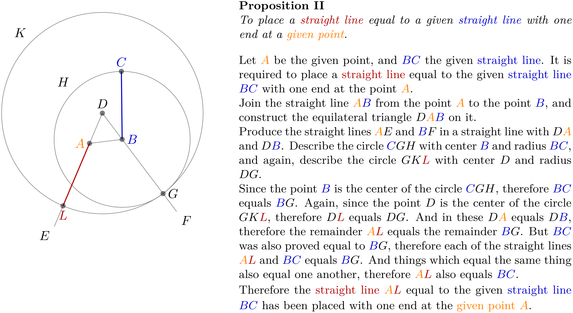
4.2 Book I, Proposition II
The second proposition in the Elements is the following:
4.2.1 Using Partway Calculations for the Construction of D
Euclid’s construction starts with “referencing” Proposition I for the construction of the point \(D\). Now, while we could simply repeat the construction, it seems a bit bothersome that one has to draw all these circles and do all these complicated constructions.
For this reason, TikZ supports some simplifications. First, there is a simple syntax for computing a point that is “partway” on a line from \(p\) to \(q\): You place these two points in a coordinate calculation – remember, they start with ($ and end with $) – and then combine them using !⟨part⟩!. A ⟨part⟩ of 0 refers to the first coordinate, a ⟨part⟩ of 1 refers to the second coordinate, and a value in between refers to a point on the line from \(p\) to \(q\). Thus, the syntax is similar to the xcolor syntax for mixing colors.
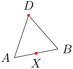
Here is the computation of the point in the middle of the line \(AB\):

                \usetikzlibrary {calc}

                \begin{tikzpicture}

                  \coordinate [label=left:$A$]  (A) at
                (0,0);

                  \coordinate [label=right:$B$] (B) at
                (1.25,0.25);

                  \draw (A) --
                (B);

                  \node [fill=red,inner sep=1pt,label=below:$X$] (X) at
                ($ (A)!.5!(B) $) {};

                \end{tikzpicture}
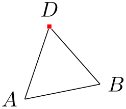
The computation of the point \(D\) in Euclid’s second proposition is a bit more complicated. It can be expressed as follows: Consider the line from \(X\) to \(B\). Suppose we rotate this line around \(X\) for 90\(^\circ \) and then stretch it by a factor of \(\sin (60^\circ ) \cdot 2\). This yields the desired point \(D\). We can do the stretching using the partway modifier above, for the rotation we need a new modifier: the rotation modifier. The idea is that the second coordinate in a partway computation can be prefixed by an angle. Then the partway point is computed normally (as if no angle were given), but the resulting point is rotated by this angle around the first point.
                \usetikzlibrary {calc}

                \begin{tikzpicture}

                  \coordinate [label=left:$A$]  (A) at
                (0,0);

                  \coordinate [label=right:$B$] (B) at
                (1.25,0.25);

                  \draw (A) --
                (B);

                  \node [fill=red,inner sep=1pt,label=below:$X$] (X) at
                ($ (A)!.5!(B) $) {};

                  \node [fill=red,inner sep=1pt,label=above:$D$] (D) at

                    ($ (X) !
                {sin(60)*2} !
                90:(B) $) {};

                  \draw (A) --
                (D) --
                (B);

                \end{tikzpicture}
Finally, it is not necessary to explicitly name the point \(X\). Rather, again like in the xcolor package, it is possible to chain partway modifiers:
                \usetikzlibrary {calc}

                \begin{tikzpicture}

                  \coordinate [label=left:$A$]  (A) at
                (0,0);

                  \coordinate [label=right:$B$] (B) at
                (1.25,0.25);

                  \draw (A) --
                (B);

                  \node [fill=red,inner sep=1pt,label=above:$D$] (D) at

                    ($ (A) !
                .5 !
                (B) !
                {sin(60)*2} !
                90:(B) $) {};

                  \draw (A) --
                (D) --
                (B);

                \end{tikzpicture}
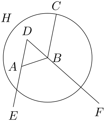
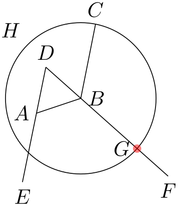
4.2.2 Intersecting a Line and a Circle
The next step in the construction is to draw a circle around \(B\) through \(C\), which is easy enough to do using the circle through option. Extending the lines \(DA\) and \(DB\) can be done using partway calculations, but this time with a part value outside the range \([0,1]\):
                \usetikzlibrary {calc,through}

                \begin{tikzpicture}

                  \coordinate [label=left:$A$]  (A) at
                (0,0);

                  \coordinate [label=right:$B$] (B) at
                (0.75,0.25);

                  \coordinate [label=above:$C$] (C) at
                (1,1.5);

                  \draw (A) --
                (B) --
                (C);

                  \coordinate [label=above:$D$] (D) at

                    ($ (A) !
                .5 !
                (B) !
                {sin(60)*2} !
                90:(B) $) {};

                  \node (H) [label=135:$H$,draw,circle through=(C)] at
                (B) {};

                  \draw (D) --
                ($ (D) !
                3.5
                !
                (B) $) coordinate [label=below:$F$] (F);

                  \draw (D) --
                ($ (D) !
                2.5
                !
                (A) $) coordinate [label=below:$E$] (E);

                \end{tikzpicture}
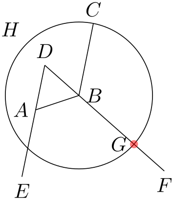
We now face the problem of finding the point \(G\), which is the intersection of the line \(BF\) and the circle \(H\). One way is to use yet another variant of the partway computation: Normally, a partway computation has the form ⟨p⟩!⟨factor⟩!⟨q⟩, resulting in the point \((1-\meta {factor})\meta {p} + \meta {factor}\meta {q}\). Alternatively, instead of ⟨factor⟩ you can also use a ⟨dimension⟩ between the points. In this case, you get the point that is ⟨dimension⟩ away from ⟨p⟩ on the straight line to ⟨q⟩.
We know that the point \(G\) is on the way from \(B\) to \(F\). The distance is given by the radius of the circle \(H\). Here is the code for computing \(H\):
                \usetikzlibrary {calc,through}

                \begin{tikzpicture}

                  \coordinate [label=left:$A$]  (A) at
                (0,0);

                  \coordinate [label=right:$B$] (B) at
                (0.75,0.25);

                  \coordinate [label=above:$C$] (C) at
                (1,1.5);

                  \draw (A) --
                (B) --
                (C);

                  \coordinate [label=above:$D$] (D) at

                    ($ (A) !
                .5 !
                (B) !
                {sin(60)*2} !
                90:(B) $) {};

                  \draw (D) --
                ($ (D) !
                3.5
                !
                (B) $) coordinate [label=below:$F$] (F);

                  \draw (D) --
                ($ (D) !
                2.5
                !
                (A) $) coordinate [label=below:$E$] (E);

                  \node (H) [label=135:$H$,draw,circle through=(C)] at
                (B) {};

                  \path let
                \p1 =
                ($ (B) -
                (C) $) in

                    coordinate
                [label=left:$G$] (G) at
                ($ (B) !
                veclen(\x1,\y1) !
                (F) $);

                  \fill[red,opacity=.5] (G) circle
                (2pt);

                \end{tikzpicture}
However, there is a simpler way: We can simply name the path of the circle and of the line in question and then use name intersections to compute the intersections.
                \usetikzlibrary {calc,intersections,through}

                \begin{tikzpicture}

                  \coordinate [label=left:$A$]  (A) at
                (0,0);

                  \coordinate [label=right:$B$] (B) at
                (0.75,0.25);

                  \coordinate [label=above:$C$] (C) at
                (1,1.5);

                  \draw (A) --
                (B) --
                (C);

                  \coordinate [label=above:$D$] (D) at

                    ($ (A) !
                .5 !
                (B) !
                {sin(60)*2} !
                90:(B) $) {};

                  \draw (D) --
                ($ (D) !
                3.5
                !
                (B) $) coordinate [label=below:$F$] (F);

                  \draw (D) --
                ($ (D) !
                2.5
                !
                (A) $) coordinate [label=below:$E$] (E);

                  \node (H) [name path=H,label=135:$H$,draw,circle through=(C)] at
                (B) {};

                  \path [name path=B--F] (B) --
                (F);

                  \path [name intersections={of=H and B--F,by={[label=left:$G$]G}}];

                  \fill[red,opacity=.5] (G) circle
                (2pt);

                \end{tikzpicture}
4.2.3 The Complete Code
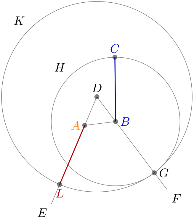
                \usetikzlibrary {calc,intersections,through}

                \begin{tikzpicture}[thick,help lines/.style={thin,draw=black!50}]

                  \def\A{\textcolor{orange}{$A$}}   \def\B{\textcolor{input}{$B$}}

                  \def\C{\textcolor{input}{$C$}}    \def\D{$D$}

                  \def\E{$E$}                       \def\F{$F$}

                  \def\G{$G$}                       \def\H{$H$}

                  \def\K{$K$}                       \def\L{\textcolor{output}{$L$}}


                  \colorlet{input}{blue!80!black}    \colorlet{output}{red!70!black}


                  \coordinate [label=left:\A]  (A) at
                ($ (0,0) +
                .1*(rand,rand) $);

                  \coordinate [label=right:\B] (B) at
                ($ (1,0.2) +
                .1*(rand,rand) $);

                  \coordinate [label=above:\C] (C) at
                ($ (1,2) +
                .1*(rand,rand) $);


                  \draw [input] (B) --
                (C);

                  \draw [help lines] (A) --
                (B);


                  \coordinate [label=above:\D] (D) at
                ($ (A)!.5!(B) !
                {sin(60)*2} !
                90:(B) $);


                  \draw [help lines] (D) --
                ($ (D)!3.75!(A) $) coordinate [label=-135:\E] (E);

                  \draw [help lines] (D) --
                ($ (D)!3.75!(B) $) coordinate [label=-45:\F] (F);


                  \node (H) at
                (B) [name path=H,help lines,circle through=(C),draw,label=135:\H] {};

                  \path [name path=B--F] (B) --
                (F);

                  \path [name intersections={of=H and B--F,by={[label=right:\G]G}}];


                  \node (K) at
                (D) [name path=K,help lines,circle through=(G),draw,label=135:\K] {};

                  \path [name path=A--E] (A) --
                (E);

                  \path [name intersections={of=K and A--E,by={[label=below:\L]L}}];


                  \draw [output] (A) --
                (L);


                  \foreach \point in
                {A,B,C,D,G,L}

                    \fill [black,opacity=.5] (\point) circle
                (2pt);


                  % \node ...

                \end{tikzpicture}