TikZ and PGF Manual
Tutorials and Guidelines
3 Tutorial: A Petri-Net for Hagen
In this second tutorial we explore the node mechanism of TikZ and pgf.
Hagen must give a talk tomorrow about his favorite formalism for distributed systems: Petri nets! Hagen used to give his talks using a blackboard and everyone seemed to be perfectly content with this. Unfortunately, his audience has been spoiled recently with fancy projector-based presentations and there seems to be a certain amount of peer pressure that his Petri nets should also be drawn using a graphic program. One of the professors at his institute recommends TikZ for this and Hagen decides to give it a try.
3.1 Problem Statement
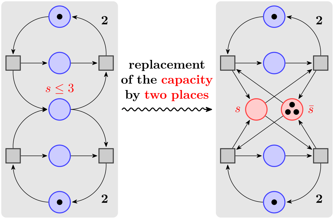
For his talk, Hagen wishes to create a graphic that demonstrates how a net with place capacities can be simulated by a net without capacities. The graphic should look like this, ideally:
3.2 Setting up the Environment
For the picture Hagen will need to load the TikZ package as did Karl in the previous tutorial. However, Hagen will also need to load some additional library packages that Karl did not need. These library packages contain additional definitions like extra arrow tips that are typically not needed in a picture and that need to be loaded explicitly.
Hagen will need to load several libraries: The arrows.meta library for the special arrow tip used in the graphic, the decorations.pathmorphing library for the “snaking line” in the middle, the backgrounds library for the two rectangular areas that are behind the two main parts of the picture, the fit library to easily compute the sizes of these rectangles, and the positioning library for placing nodes relative to other nodes.
3.2.1 Setting up the Environment in LaTeX
When using LaTeX use:
                \documentclass{article} % say


                \usepackage{tikz}

                \usetikzlibrary{arrows.meta,decorations.pathmorphing,backgrounds,positioning,fit,petri}


                \begin{document}

                \begin{tikzpicture}

                  \draw (0,0) --
                (1,1);

                \end{tikzpicture}

                \end{document}
3.2.2 Setting up the Environment in Plain TeX
When using plain TeX use:
                %% Plain TeX file

                \input tikz.tex

                \usetikzlibrary{arrows.meta,decorations.pathmorphing,backgrounds,positioning,fit,petri}

                \baselineskip=12pt

                \hsize=6.3truein

                \vsize=8.7truein

                \tikzpicture

                  \draw (0,0) --
                (1,1);

                \endtikzpicture

                \bye
3.2.3 Setting up the Environment in ConTeXt
When using ConTeXt, use:
                %% ConTeXt file

                \usemodule[tikz]

                \usetikzlibrary[arrows.meta,decorations.pathmorphing,backgrounds,positioning,fit,petri]


                \starttext

                  \starttikzpicture

                    \draw (0,0) --
                (1,1);

                  \stoptikzpicture

                \stoptext
3.3 Introduction to Nodes
In principle, we already know how to create the graphics that Hagen desires (except perhaps for the snaked line, we will come to that): We start with big light gray rectangle and then add lots of circles and small rectangle, plus some arrows.
However, this approach has numerous disadvantages: First, it is hard to change anything at a later stage. For example, if we decide to add more places to the Petri nets (the circles are called places in Petri net theory), all of the coordinates change and we need to recalculate everything. Second, it is hard to read the code for the Petri net as it is just a long and complicated list of coordinates and drawing commands – the underlying structure of the Petri net is lost.
Fortunately, TikZ offers a powerful mechanism for avoiding the above problems: nodes. We already came across nodes in the previous tutorial, where we used them to add labels to Karl’s graphic. In the present tutorial we will see that nodes are much more powerful.
A node is a small part of a picture. When a node is created, you provide a position where the node should be drawn and a shape. A node of shape circle will be drawn as a circle, a node of shape rectangle as a rectangle, and so on. A node may also contain some text, which is why Karl used nodes to show text. Finally, a node can get a name for later reference.
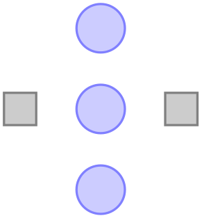
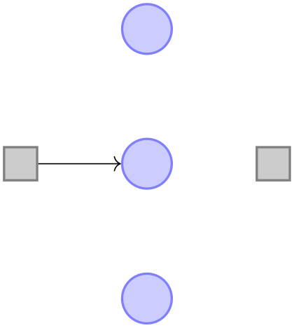
In Hagen’s picture we will use nodes for the places and for the transitions of the Petri net (the places are the circles, the transitions are the rectangles). Let us start with the upper half of the left Petri net. In this upper half we have three places and two transitions. Instead of drawing three circles and two rectangles, we use three nodes of shape circle and two nodes of shape rectangle.
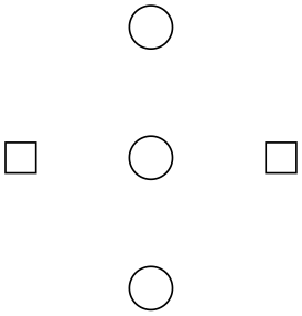
Hagen notes that this does not quite look like the final picture, but it seems like a good first step.
Let us have a more detailed look at the code. The whole picture consists of a single path. Ignoring the node operations, there is not much going on in this path: It is just a sequence of coordinates with nothing “happening” between them. Indeed, even if something were to happen like a line-to or a curve-to, the \path command would not “do” anything with the resulting path. So, all the magic must be in the node commands.
In the previous tutorial we learned that a node will add a piece of text at the last coordinate. Thus, each of the five nodes is added at a different position. In the above code, this text is empty (because of the empty {}). So, why do we see anything at all? The answer is the draw option for the node operation: It causes the “shape around the text” to be drawn.
So, the code (0,2) node [shape=circle,draw] {} means the following: “In the main path, add a move-to to the coordinate (0,2). Then, temporarily suspend the construction of the main path while the node is built. This node will be a circle around an empty text. This circle is to be drawn, but not filled or otherwise used. Once this whole node is constructed, it is saved until after the main path is finished. Then, it is drawn.” The following (0,1) node [shape=circle,draw] {} then has the following effect: “Continue the main path with a move-to to (0,1). Then construct a node at this position also. This node is also shown after the main path is finished.” And so on.
3.4 Placing Nodes Using the At Syntax
Hagen now understands how the node operation adds nodes to the path, but it seems a bit silly to create a path using the \path operation, consisting of numerous superfluous move-to operations, only to place nodes. He is pleased to learn that there are ways to add nodes in a more sensible manner.
First, the node operation allows one to add at (⟨coordinate⟩) in order to directly specify where the node should be placed, sidestepping the rule that nodes are placed on the last coordinate. Hagen can then write the following:

Now Hagen is still left with a single empty path, but at least the path no longer contains strange move-to’s. It turns out that this can be improved further: The \node command is an abbreviation for \path node, which allows Hagen to write:

Hagen likes this syntax much better than the previous one. Note that Hagen has also omitted the shape= since, like color=, TikZ allows you to omit the shape= if there is no confusion.
3.5 Using Styles
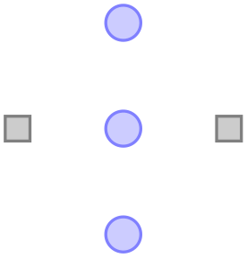
Feeling adventurous, Hagen tries to make the nodes look nicer. In the final picture, the circles and rectangle should be filled with different colors, resulting in the following code:

                \begin{tikzpicture}[thick]

                  \node at
                ( 0,2) [circle,draw=blue!50,fill=blue!20] {};

                  \node at
                ( 0,1) [circle,draw=blue!50,fill=blue!20] {};

                  \node at
                ( 0,0) [circle,draw=blue!50,fill=blue!20] {};

                  \node at
                ( 1,1) [rectangle,draw=black!50,fill=black!20] {};

                  \node at
                (-1,1) [rectangle,draw=black!50,fill=black!20] {};

                \end{tikzpicture}
While this looks nicer in the picture, the code starts to get a bit ugly. Ideally, we would like our code to transport the message “there are three places and two transitions” and not so much which filling colors should be used.
To solve this problem, Hagen uses styles. He defines a style for places and another style for transitions:
                \begin{tikzpicture}

                  [place/.style={circle,draw=blue!50,fill=blue!20,thick},

                   transition/.style={rectangle,draw=black!50,fill=black!20,thick}]

                  \node at
                ( 0,2) [place] {};

                  \node at
                ( 0,1) [place] {};

                  \node at
                ( 0,0) [place] {};

                  \node at
                ( 1,1) [transition] {};

                  \node at
                (-1,1) [transition] {};

                \end{tikzpicture}
3.6 Node Size
Before Hagen starts naming and connecting the nodes, let us first make sure that the nodes get their final appearance. They are still too small. Indeed, Hagen wonders why they have any size at all, after all, the text is empty. The reason is that TikZ automatically adds some space around the text. The amount is set using the option inner sep. So, to increase the size of the nodes, Hagen could write:
                \begin{tikzpicture}

                  [inner sep=2mm,

                   place/.style={circle,draw=blue!50,fill=blue!20,thick},

                   transition/.style={rectangle,draw=black!50,fill=black!20,thick}]

                  \node at
                ( 0,2) [place] {};

                  \node at
                ( 0,1) [place] {};

                  \node at
                ( 0,0) [place] {};

                  \node at
                ( 1,1) [transition] {};

                  \node at
                (-1,1) [transition] {};

                \end{tikzpicture}
However, this is not really the best way to achieve the desired effect. It is much better to use the minimum size option instead. This option allows Hagen to specify a minimum size that the node should have. If the node actually needs to be bigger because of a longer text, it will be larger, but if the text is empty, then the node will have minimum size. This option is also useful to ensure that several nodes containing different amounts of text have the same size. The options minimum height and minimum width allow you to specify the minimum height and width independently.
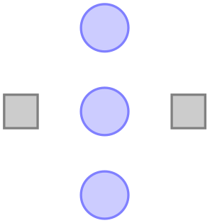
So, what Hagen needs to do is to provide minimum size for the nodes. To be on the safe side, he also sets inner sep=0pt. This ensures that the nodes will really have size minimum size and not, for very small minimum sizes, the minimal size necessary to encompass the automatically added space.

                \begin{tikzpicture}

                  [place/.style={circle,draw=blue!50,fill=blue!20,thick,

                                 inner sep=0pt,minimum size=6mm},

                   transition/.style={rectangle,draw=black!50,fill=black!20,thick,

                                      inner sep=0pt,minimum size=4mm}]

                  \node at
                ( 0,2) [place] {};

                  \node at
                ( 0,1) [place] {};

                  \node at
                ( 0,0) [place] {};

                  \node at
                ( 1,1) [transition] {};

                  \node at
                (-1,1) [transition] {};

                \end{tikzpicture}
3.7 Naming Nodes
Hagen’s next aim is to connect the nodes using arrows. This seems like a tricky business since the arrows should not start in the middle of the nodes, but somewhere on the border and Hagen would very much like to avoid computing these positions by hand.
Fortunately, pgf will perform all the necessary calculations for him. However, he first has to assign names to the nodes so that he can reference them later on.
There are two ways to name a node. The first is to use the name= option. The second method is to write the desired name in parentheses after the node operation. Hagen thinks that this second method seems strange, but he will soon change his opinion.

                % ... set up styles

                \begin{tikzpicture}

                  \node (waiting 1)      at
                ( 0,2) [place] {};

                  \node (critical 1)     at
                ( 0,1) [place] {};

                  \node (semaphore)      at
                ( 0,0) [place] {};

                  \node (leave critical) at
                ( 1,1) [transition] {};

                  \node (enter critical) at
                (-1,1) [transition] {};

                \end{tikzpicture}
Hagen is pleased to note that the names help in understanding the code. Names for nodes can be pretty arbitrary, but they should not contain commas, periods, parentheses, colons, and some other special characters. However, they can contain underscores and hyphens.
The syntax for the node operation is quite liberal with respect to the order in which node names, the at specifier, and the options must come. Indeed, you can even have multiple option blocks between the node and the text in curly braces, they accumulate. You can rearrange them arbitrarily and perhaps the following might be preferable:
                \begin{tikzpicture}

                  \node[place]      (waiting 1)      at
                ( 0,2) {};

                  \node[place]      (critical 1)     at
                ( 0,1) {};

                  \node[place]      (semaphore)      at
                ( 0,0) {};

                  \node[transition] (leave critical) at
                ( 1,1) {};

                  \node[transition] (enter critical) at
                (-1,1) {};

                \end{tikzpicture}
3.8 Placing Nodes Using Relative Placement
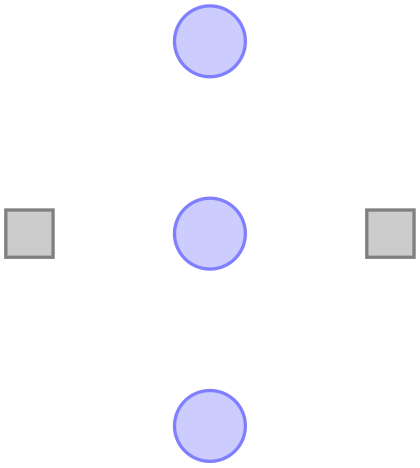
Although Hagen still wishes to connect the nodes, he first wishes to address another problem again: The placement of the nodes. Although he likes the at syntax, in this particular case he would prefer placing the nodes “relative to each other”. So, Hagen would like to say that the critical 1 node should be below the waiting 1 node, wherever the waiting 1 node might be. There are different ways of achieving this, but the nicest one in Hagen’s case is the below option:
                \usetikzlibrary {positioning}

                \begin{tikzpicture}

                  \node[place]      (waiting)                            {};

                  \node[place]      (critical)       [below=of waiting]  {};

                  \node[place]      (semaphore)      [below=of critical] {};

                  \node[transition] (leave critical) [right=of critical] {};

                  \node[transition] (enter critical) [left=of critical]  {};

                \end{tikzpicture}
With the positioning library loaded, when an option like below is followed by of, then the position of the node is shifted in such a manner that it is placed at the distance node distance in the specified direction of the given direction. The node distance is either the distance between the centers of the nodes (when the on grid option is set to true) or the distance between the borders (when the on grid option is set to false, which is the default).
Even though the above code has the same effect as the earlier code, Hagen can pass it to his colleagues who will be able to just read and understand it, perhaps without even having to see the picture.
3.9 Adding Labels Next to Nodes
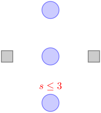
Before we have a look at how Hagen can connect the nodes, let us add the capacity “\(s \le 3\)” to the bottom node. For this, two approaches are possible:
-
1. Hagen can just add a new node above the north anchor of the semaphore node.
                    \usetikzlibrary {positioning}

                    \begin{tikzpicture}

                      \node[place]      (waiting)                            {};

                      \node[place]      (critical)       [below=of waiting]  {};

                      \node[place]      (semaphore)      [below=of critical] {};

                      \node[transition] (leave critical) [right=of critical] {};

                      \node[transition] (enter critical) [left=of critical]  {};


                      \node [red,above] at
                    (semaphore.north) {$s\le 3$};

                    \end{tikzpicture}
This is a general approach that will “always work”.
-
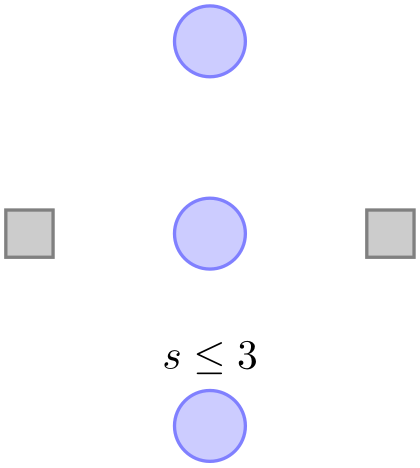
2. Hagen can use the special label option. This option is given to a node and it causes another node to be added next to the node where the option is given. Here is the idea: When we construct the semaphore node, we wish to indicate that we want another node with the capacity above it. For this, we use the option label=above:$s\le 3$. This option is interpreted as follows: We want a node above the semaphore node and this node should read “\(s \le 3\)”. Instead of above we could also use things like below left before the colon or a number like 60.
                    \usetikzlibrary {positioning}

                    \begin{tikzpicture}

                      \node[place]      (waiting)                            {};

                      \node[place]      (critical)       [below=of waiting]  {};

                      \node[place]      (semaphore)      [below=of critical,

                                                          label=above:$s\le3$] {};

                      \node[transition] (leave critical) [right=of critical] {};

                      \node[transition] (enter critical) [left=of critical]  {};

                    \end{tikzpicture}
It is also possible to give multiple label options, this causes multiple labels to be drawn.

Hagen is not fully satisfied with the label option since the label is not red. To achieve this, he has two options: First, he can redefine the every label style. Second, he can add options to the label’s node. These options are given following the label=, so he would write label=[red]above:$s\le3$. However, this does not quite work since TeX thinks that the ] closes the whole option list of the semaphore node. So, Hagen has to add braces and writes label={[red]above:$s\le3$}. Since this looks a bit ugly, Hagen decides to redefine the every label style.

                    \usetikzlibrary {positioning}

                    \begin{tikzpicture}[every label/.style={red}]

                      \node[place]      (waiting)                            {};

                      \node[place]      (critical)       [below=of waiting]  {};

                      \node[place]      (semaphore)      [below=of critical,

                                                          label=above:$s\le3$] {};

                      \node[transition] (leave critical) [right=of critical] {};

                      \node[transition] (enter critical) [left=of critical]  {};

                    \end{tikzpicture}
3.10 Connecting Nodes
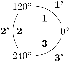
It is now high time to connect the nodes. Let us start with something simple, namely with the straight line from enter critical to critical. We want this line to start at the right side of enter critical and to end at the left side of critical. For this, we can use the anchors of the nodes. Every node defines a whole bunch of anchors that lie on its border or inside it. For example, the center anchor is at the center of the node, the west anchor is on the left of the node, and so on. To access the coordinate of a node, we use a coordinate that contains the node’s name followed by a dot, followed by the anchor’s name:
                \usetikzlibrary {positioning}

                \begin{tikzpicture}

                  \node[place]      (waiting)                            {};

                  \node[place]      (critical)       [below=of waiting]  {};

                  \node[place]      (semaphore)      [below=of critical] {};

                  \node[transition] (leave critical) [right=of critical] {};

                  \node[transition] (enter critical) [left=of critical]  {};

                  \draw [->] (enter critical.east) --
                (critical.west);

                \end{tikzpicture}
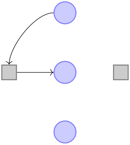
Next, let us tackle the curve from waiting to enter critical. This can be specified using curves and controls:
                \usetikzlibrary {positioning}

                \begin{tikzpicture}

                  \node[place]      (waiting)                            {};

                  \node[place]      (critical)       [below=of waiting]  {};

                  \node[place]      (semaphore)      [below=of critical] {};

                  \node[transition] (leave critical) [right=of critical] {};

                  \node[transition] (enter critical) [left=of critical]  {};

                  \draw [->] (enter critical.east) --
                (critical.west);

                  \draw [->] (waiting.west) .. controls
                +(left:5mm) and
                +(up:5mm)

                                            .. (enter critical.north);

                \end{tikzpicture}
Hagen sees how he can now add all his edges, but the whole process seems a but awkward and not very flexible. Again, the code seems to obscure the structure of the graphic rather than showing it.
So, let us start improving the code for the edges. First, Hagen can leave out the anchors:

                \usetikzlibrary {positioning}

                \begin{tikzpicture}

                  \node[place]      (waiting)                            {};

                  \node[place]      (critical)       [below=of waiting]  {};

                  \node[place]      (semaphore)      [below=of critical] {};

                  \node[transition] (leave critical) [right=of critical] {};

                  \node[transition] (enter critical) [left=of critical]  {};

                  \draw [->] (enter critical) --
                (critical);

                  \draw [->] (waiting) .. controls
                +(left:8mm) and
                +(up:8mm)

                                       .. (enter critical);

                \end{tikzpicture}
Hagen is a bit surprised that this works. After all, how did TikZ know that the line from enter critical to critical should actually start on the borders? Whenever TikZ encounters a whole node name as a “coordinate”, it tries to “be smart” about the anchor that it should choose for this node. Depending on what happens next, TikZ will choose an anchor that lies on the border of the node on a line to the next coordinate or control point. The exact rules are a bit complex, but the chosen point will usually be correct – and when it is not, Hagen can still specify the desired anchor by hand.
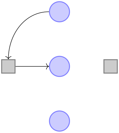
Hagen would now like to simplify the curve operation somehow. It turns out that this can be accomplished using a special path operation: the to operation. This operation takes many options (you can even define new ones yourself). One pair of options is useful for Hagen: The pair in and out. These options take angles at which a curve should leave or reach the start or target coordinates. Without these options, a straight line is drawn:
                \usetikzlibrary {positioning}

                \begin{tikzpicture}

                  \node[place]      (waiting)                            {};

                  \node[place]      (critical)       [below=of waiting]  {};

                  \node[place]      (semaphore)      [below=of critical] {};

                  \node[transition] (leave critical) [right=of critical] {};

                  \node[transition] (enter critical) [left=of critical]  {};

                  \draw [->] (enter critical) to
                                (critical);

                  \draw [->] (waiting)        to
                [out=180,in=90] (enter critical);

                \end{tikzpicture}
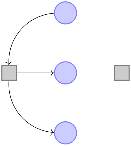
There is another option for the to operation, that is even better suited to Hagen’s problem: The bend right option. This option also takes an angle, but this angle only specifies the angle by which the curve is bent to the right:

                \usetikzlibrary {positioning}

                \begin{tikzpicture}

                  \node[place]      (waiting)                            {};

                  \node[place]      (critical)       [below=of waiting]  {};

                  \node[place]      (semaphore)      [below=of critical] {};

                  \node[transition] (leave critical) [right=of critical] {};

                  \node[transition] (enter critical) [left=of critical]  {};

                  \draw [->] (enter critical) to
                                (critical);

                  \draw [->] (waiting)        to
                [bend right=45] (enter critical);

                  \draw [->] (enter critical) to
                [bend right=45] (semaphore);

                \end{tikzpicture}
It is now time for Hagen to learn about yet another way of specifying edges: Using the edge path operation. This operation is very similar to the to operation, but there is one important difference: Like a node the edge generated by the edge operation is not part of the main path, but is added only later. This may not seem very important, but it has some nice consequences. For example, every edge can have its own arrow tips and its own color and so on and, still, all the edges can be given on the same path. This allows Hagen to write the following:
                \usetikzlibrary {positioning}

                \begin{tikzpicture}

                  \node[place]      (waiting)                            {};

                  \node[place]      (critical)       [below=of waiting]  {};

                  \node[place]      (semaphore)      [below=of critical] {};

                  \node[transition] (leave critical) [right=of critical] {};

                  \node[transition] (enter critical) [left=of critical]  {}

                    edge
                [->]               (critical)

                    edge
                [<-,bend left=45]  (waiting)

                    edge
                [->,bend right=45] (semaphore);

                \end{tikzpicture}
Each edge caused a new path to be constructed, consisting of a to between the node enter critical and the node following the edge command.
The finishing touch is to introduce two styles pre and post and to use the bend angle=45 option to set the bend angle once and for all:

                \usetikzlibrary {arrows.meta,positioning}

                % Styles place and transition as before

                \begin{tikzpicture}

                  [bend angle=45,

                   pre/.style={<-,shorten <=1pt,>={Stealth[round]},semithick},

                   post/.style={->,shorten >=1pt,>={Stealth[round]},semithick}]


                  \node[place]      (waiting)                            {};

                  \node[place]      (critical)       [below=of waiting]  {};

                  \node[place]      (semaphore)      [below=of critical] {};


                  \node[transition] (leave critical) [right=of critical] {}

                    edge
                [pre]             (critical)

                    edge
                [post,bend right] (waiting)

                    edge
                [pre, bend left]  (semaphore);

                  \node[transition] (enter critical) [left=of critical]  {}

                    edge
                [post]            (critical)

                    edge
                [pre, bend left]  (waiting)

                    edge
                [post,bend right] (semaphore);

                \end{tikzpicture}
3.11 Adding Labels Next to Lines
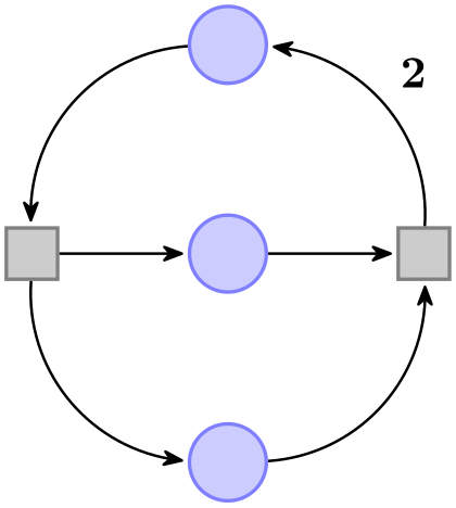
The next thing that Hagen needs to add is the “\(2\)” at the arcs. For this Hagen can use TikZ’s automatic node placement: By adding the option auto, TikZ will position nodes on curves and lines in such a way that they are not on the curve but next to it. Adding swap will mirror the label with respect to the line. Here is a general example:
What is happening here? The nodes are given somehow inside the to operation! When this is done, the node is placed on the middle of the curve or line created by the to operation. The auto option then causes the node to be moved in such a way that it does not lie on the curve, but next to it. In the example we provide even two nodes on each to operation.
For Hagen that auto option is not really necessary since the two “2” labels could also easily be placed “by hand”. However, in a complicated plot with numerous edges automatic placement can be a blessing.
                \usetikzlibrary {arrows.meta,positioning}

                % Styles as before

                \begin{tikzpicture}[bend angle=45]

                  \node[place]      (waiting)                            {};

                  \node[place]      (critical)       [below=of waiting]  {};

                  \node[place]      (semaphore)      [below=of critical] {};


                  \node[transition] (leave critical) [right=of critical] {}

                    edge
                [pre]                                 (critical)

                    edge
                [post,bend right] node[auto,swap] {2} (waiting)

                    edge
                [pre, bend left]                      (semaphore);

                  \node[transition] (enter critical) [left=of critical]  {}

                    edge
                [post]                                (critical)

                    edge
                [pre, bend left]                      (waiting)

                    edge
                [post,bend right]                     (semaphore);

                \end{tikzpicture}
3.12 Adding the Snaked Line and Multi-Line Text
With the node mechanism Hagen can now easily create the two Petri nets. What he is unsure of is how he can create the snaked line between the nets.
For this he can use a decoration. To draw the snaked line, Hagen only needs to set the two options decoration=snake and decorate on the path. This causes all lines of the path to be replaced by snakes. It is also possible to use snakes only in certain parts of a path, but Hagen will not need this.

                \usetikzlibrary {decorations.pathmorphing}

                \begin{tikzpicture}

                  \draw [->,decorate,decoration=snake] (0,0) --
                (2,0);

                \end{tikzpicture}
Well, that does not look quite right, yet. The problem is that the snake happens to end exactly at the position where the arrow begins. Fortunately, there is an option that helps here. Also, the snake should be a bit smaller, which can be influenced by even more options.

                \usetikzlibrary {decorations.pathmorphing}

                \begin{tikzpicture}

                  \draw [->,decorate,

                     decoration={snake,amplitude=.4mm,segment length=2mm,post length=1mm}]

                    (0,0) --
                (3,0);

                \end{tikzpicture}
Now Hagen needs to add the text above the snake. This text is a bit challenging since it is a multi-line text. Hagen has two options for this: First, he can specify an align=center and then use the \\ command to enforce the line breaks at the desired positions.

                \usetikzlibrary {decorations.pathmorphing}

                \begin{tikzpicture}

                  \draw [->,decorate,

                      decoration={snake,amplitude=.4mm,segment length=2mm,post length=1mm}]

                    (0,0) --
                (3,0)

                    node
                [above,align=center,midway]

                    {

                      replacement
                of\\

                      the
                \textcolor{red}{capacity}\\

                      by
                \textcolor{red}{two
                places}

                    };

                \end{tikzpicture}
Instead of specifying the line breaks “by hand”, Hagen can also specify a width for the text and let TeX perform the line breaking for him:

                \usetikzlibrary {decorations.pathmorphing}

                \begin{tikzpicture}

                  \draw [->,decorate,

                      decoration={snake,amplitude=.4mm,segment length=2mm,post length=1mm}]

                    (0,0) --
                (3,0)

                    node
                [above,text width=3cm,align=center,midway]

                    {

                      replacement
                of
                the
                \textcolor{red}{capacity} by

                      \textcolor{red}{two
                places}

                    };

                \end{tikzpicture}
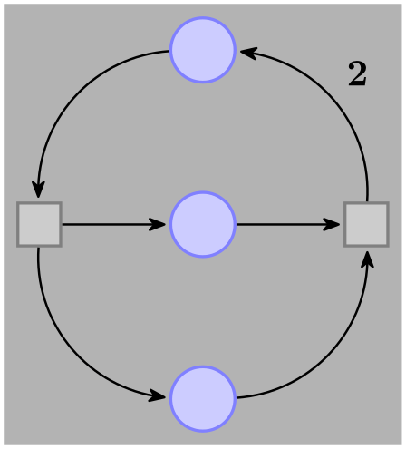
3.13 Using Layers: The Background Rectangles
Hagen still needs to add the background rectangles. These are a bit tricky: Hagen would like to draw the rectangles after the Petri nets are finished. The reason is that only then can he conveniently refer to the coordinates that make up the corners of the rectangle. If Hagen draws the rectangle first, then he needs to know the exact size of the Petri net – which he does not.
The solution is to use layers. When the backgrounds library is loaded, Hagen can put parts of his picture inside a scope with the on background layer option. Then this part of the picture becomes part of the layer that is given as an argument to this environment. When the {tikzpicture} environment ends, the layers are put on top of each other, starting with the background layer. This causes everything drawn on the background layer to be behind the main text.
The next tricky question is, how big should the rectangle be? Naturally, Hagen can compute the size “by hand” or using some clever observations concerning the \(x\)- and \(y\)-coordinates of the nodes, but it would be nicer to just have TikZ compute a rectangle into which all the nodes “fit”. For this, the fit library can be used. It defines the fit options, which, when given to a node, causes the node to be resized and shifted such that it exactly covers all the nodes and coordinates given as parameters to the fit option.
                \usetikzlibrary {arrows.meta,backgrounds,fit,positioning}

                % Styles as before

                \begin{tikzpicture}[bend angle=45]

                  \node[place]      (waiting)                            {};

                  \node[place]      (critical)       [below=of waiting]  {};

                  \node[place]      (semaphore)      [below=of critical] {};


                  \node[transition] (leave critical) [right=of critical] {}

                    edge
                [pre]                                 (critical)

                    edge
                [post,bend right] node[auto,swap] {2} (waiting)

                    edge
                [pre, bend left]                      (semaphore);

                  \node[transition] (enter critical) [left=of critical]  {}

                    edge
                [post]                                (critical)

                    edge
                [pre, bend left]                      (waiting)

                    edge
                [post,bend right]                     (semaphore);


                  \begin{scope}[on background layer]

                    \node [fill=black!30,fit=(waiting) (critical) (semaphore)

                               (leave critical) (enter critical)] {};

                  \end{scope}

                \end{tikzpicture}
3.14 The Complete Code
Hagen has now finally put everything together. Only then does he learn that there is already a library for drawing Petri nets! It turns out that this library mainly provides the same definitions as Hagen did. For example, it defines a place style in a similar way as Hagen did. Adjusting the code so that it uses the library shortens Hagen code a bit, as shown in the following.
First, Hagen needs less style definitions, but he still needs to specify the colors of places and transitions.
                \begin{tikzpicture}

                  [node distance=1.3cm,on grid,>={Stealth[round]},bend angle=45,auto,

                   every place/.style= {minimum size=6mm,thick,draw=blue!75,fill=blue!20},

                   every transition/.style={thick,draw=black!75,fill=black!20},

                   red place/.style= {place,draw=red!75,fill=red!20},

                   every label/.style= {red}]
Now comes the code for the nets:

                \usetikzlibrary {arrows.meta,petri,positioning}

                   \node [place,tokens=1] (w1)                                    {};

                   \node [place]          (c1) [below=of w1]                      {};

                   \node [place]          (s)  [below=of c1,label=above:$s\le 3$] {};

                   \node [place]          (c2) [below=of s]                       {};

                   \node [place,tokens=1] (w2) [below=of c2]                      {};


                   \node [transition] (e1) [left=of c1] {}

                     edge
                [pre,bend left]                  (w1)

                     edge
                [post,bend right]                (s)

                     edge
                [post]                           (c1);

                   \node [transition] (e2) [left=of c2] {}

                     edge
                [pre,bend right]                 (w2)

                     edge
                [post,bend left]                 (s)

                     edge
                [post]                           (c2);

                   \node [transition] (l1) [right=of c1] {}

                     edge
                [pre]                            (c1)

                     edge
                [pre,bend left]                  (s)

                     edge
                [post,bend right] node[swap] {2} (w1);

                   \node [transition] (l2) [right=of c2] {}

                     edge
                [pre]                            (c2)

                     edge
                [pre,bend right]                 (s)

                     edge
                [post,bend left]  node {2}       (w2);

                \usetikzlibrary {arrows.meta,petri,positioning}

                  \begin{scope}[xshift=6cm]

                    \node [place,tokens=1]     (w1')                            {};

                    \node [place]              (c1') [below=of w1']             {};

                    \node [red place]          (s1') [below=of c1',xshift=-5mm]

                            [label=left:$s$]                                    {};

                    \node [red place,tokens=3] (s2') [below=of c1',xshift=5mm]

                            [label=right:$\bar s$]                              {};

                    \node [place]              (c2') [below=of s1',xshift=5mm]  {};

                    \node [place,tokens=1]     (w2') [below=of c2']             {};


                    \node [transition] (e1') [left=of c1'] {}

                      edge
                [pre,bend left]                  (w1')

                      edge
                [post]                           (s1')

                      edge
                [pre]                            (s2')

                      edge
                [post]                           (c1');

                    \node [transition] (e2') [left=of c2'] {}

                      edge
                [pre,bend right]                 (w2')

                      edge
                [post]                           (s1')

                      edge
                [pre]                            (s2')

                      edge
                [post]                           (c2');

                    \node [transition] (l1') [right=of c1'] {}

                      edge
                [pre]                            (c1')

                      edge
                [pre]                            (s1')

                      edge
                [post]                           (s2')

                      edge
                [post,bend right] node[swap] {2} (w1');

                    \node [transition] (l2') [right=of c2'] {}

                      edge
                [pre]                            (c2')

                      edge
                [pre]                            (s1')

                      edge
                [post]                           (s2')

                      edge
                [post,bend left]  node {2}       (w2');

                  \end{scope}
The code for the background and the snake is the following:
                  \begin{scope}[on background layer]

                    \node (r1) [fill=black!10,rounded corners,fit=(w1)(w2)(e1)(e2)(l1)(l2)] {};

                    \node (r2) [fill=black!10,rounded corners,fit=(w1')(w2')(e1')(e2')(l1')(l2')] {};

                  \end{scope}


                  \draw [shorten >=1mm,->,thick,decorate,

                         decoration={snake,amplitude=.4mm,segment length=2mm,

                                       pre=moveto,pre
                  length=1mm,post length=2mm}]

                    (r1) --
                (r2) node
                [above=1mm,midway,text width=3cm,align=center]

                      {replacement
                of
                the
                \textcolor{red}{capacity} by
                \textcolor{red}{two
                places}};

                \end{tikzpicture}