TikZ and PGF Manual
Tutorials and Guidelines
6 Tutorial: A Lecture Map for Johannes
In this tutorial we explore the tree and mind map mechanisms of TikZ.
Johannes is quite excited: For the first time he will be teaching a course all by himself during the upcoming semester! Unfortunately, the course is not on his favorite subject, which is of course Theoretical Immunology, but on Complexity Theory, but as a young academic Johannes is not likely to complain too loudly. In order to help the students get a general overview of what is going to happen during the course as a whole, he intends to draw some kind of tree or graph containing the basic concepts. He got this idea from his old professor who seems to be using these “lecture maps” with some success. Independently of the success of these maps, Johannes thinks they look quite neat.
6.1 Problem Statement
Johannes wishes to create a lecture map with the following features:
-
1. It should contain a tree or graph depicting the main concepts.
-
2. It should somehow visualize the different lectures that will be taught. Note that the lectures are not necessarily the same as the concepts since the graph may contain more concepts than will be addressed in lectures and some concepts may be addressed during more than one lecture.
-
3. The map should also contain a calendar showing when the individual lectures will be given.
-
4. The aesthetical reasons, the whole map should have a visually nice and information-rich background.
As always, Johannes will have to include the right libraries and set up the environment. Johannes is going to use the mindmap library and since he wishes to show a calendar, he will also need the calendar library. In order to put something on a background layer, it seems like a good idea to also include the backgrounds library.
6.2 Introduction to Trees
The first choice Johannes must make is whether he will organize the concepts as a tree, with root concepts and concept branches and leaf concepts, or as a general graph. The tree implicitly organizes the concepts, while a graph is more flexible. Johannes decides to compromise: Basically, the concepts will be organized as a tree. However, he will selectively add connections between concepts that are related, but which appear on different levels or branches of the tree.
Johannes starts with a tree-like list of concepts that he feels are important in Computational Complexity:
-
• Computational Problems
-
– Problem Measures
-
– Problem Aspects
-
– Problem Domains
-
– Key Problems
-
-
• Computational Models
-
– Turing Machines
-
– Random-Access Machines
-
– Circuits
-
– Binary Decision Diagrams
-
– Oracle Machines
-
– Programming in Logic
-
-
• Measuring Complexity
-
– Complexity Measures
-
– Classifying Complexity
-
– Comparing Complexity
-
– Describing Complexity
-
-
• Solving Problems
-
– Exact Algorithms
-
– Randomization
-
– Fixed-Parameter Algorithms
-
– Parallel Computation
-
– Partial Solutions
-
– Approximation
-
Johannes will surely need to modify this list later on, but it looks good as a first approximation. He will also need to add a number of subtopics (like lots of complexity classes under the topic “classifying complexity”), but he will do this as he constructs the map.
Turning the list of topics into a TikZ-tree is easy, in principle. The basic idea is that a node can have children, which in turn can have children of their own, and so on. To add a child to a node, Johannes can simply write child {⟨node⟩} right after a node. The ⟨node⟩ should, in turn, be the code for creating a node. To add another node, Johannes can use child once more, and so on. Johannes is eager to try out this construct and writes down the following:

                \tikz

                  \node {Computational
                Complexity} % root

                    child
                { node {Computational
                Problems}

                      child
                { node {Problem
                Measures} }

                      child
                { node {Problem
                Aspects} }

                      child
                { node {Problem
                Domains} }

                      child
                { node {Key
                Problems} }

                    }

                    child
                { node {Computational
                Models}

                      child
                { node {Turing
                Machines} }

                      child
                { node {Random-Access
                Machines} }

                      child
                { node {Circuits} }

                      child
                { node {Binary
                Decision
                Diagrams} }

                      child
                { node {Oracle
                Machines} }

                      child
                { node {Programming
                in
                Logic} }

                    }

                    child
                { node {Measuring
                Complexity}

                      child
                { node {Complexity
                Measures} }

                      child
                { node {Classifying
                Complexity} }

                      child
                { node {Comparing
                Complexity} }

                      child
                { node {Describing
                Complexity} }

                    }

                    child
                { node {Solving
                Problems}

                      child
                { node {Exact
                Algorithms} }

                      child
                { node {Randomization} }

                      child
                { node {Fixed-Parameter
                Algorithms} }

                      child
                { node {Parallel
                Computation} }

                      child
                { node {Partial
                Solutions} }

                      child
                { node {Approximation} }

                    };
Well, that did not quite work out as expected (although, what, exactly, did one expect?). There are two problems:
-
1. The overlap of the nodes is due to the fact that TikZ is not particularly smart when it comes to placing child nodes. Even though it is possible to configure TikZ to use rather clever placement methods, TikZ has no way of taking the actual size of the child nodes into account. This may seem strange but the reason is that the child nodes are rendered and placed one at a time, so the size of the last node is not known when the first node is being processed. In essence, you have to specify appropriate level and sibling node spacings “by hand”.
-
2. The standard computer-science-top-down rendering of a tree is rather ill-suited to visualizing the concepts. It would be better to either rotate the map by ninety degrees or, even better, to use some sort of circular arrangement.
Johannes redraws the tree, but this time with some more appropriate options set, which he found more or less by trial-and-error:
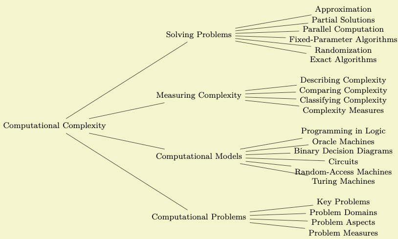
                \usetikzlibrary {trees}

                \tikz [font=\footnotesize,

                       grow=right, level 1/.style={sibling distance=6em},

                                   level 2/.style={sibling distance=1em}, level distance=5cm]

                  \node {Computational
                Complexity} % root

                    child
                { node {Computational
                Problems}

                      child
                { node {Problem
                Measures} }

                      child
                { node {Problem
                Aspects} }

                      ... % as before
Still not quite what Johannes had in mind, but he is getting somewhere.
For configuring the tree, two parameters are of particular importance: The level distance tells TikZ the distance between (the centers of) the nodes on adjacent levels or layers of a tree. The sibling distance is, as the name suggests, the distance between (the centers of) siblings of the tree.
You can globally set these parameters for a tree by simply setting them somewhere before the tree starts, but you will typically wish them to be different for different levels of the tree. In this case, you should set styles like level 1 or level 2. For the first level of the tree, the level 1 style is used, for the second level the level 2 style, and so on. You can also set the sibling and level distances only for certain nodes by passing these options to the child command as options. (Note that the options of a node command are local to the node and have no effect on the children. Also note that it is possible to specify options that do have an effect on the children. Finally note that specifying options for children “at the right place” is an arcane art and you should peruse Section 21.4 on a rainy Sunday afternoon, if you are really interested.)
The grow key is used to configure the direction in which a tree grows. You can change growth direction “in the middle of a tree” simply by changing this key for a single child or a whole level. By including the trees library you also get access to additional growth strategies such as a “circular” growth:
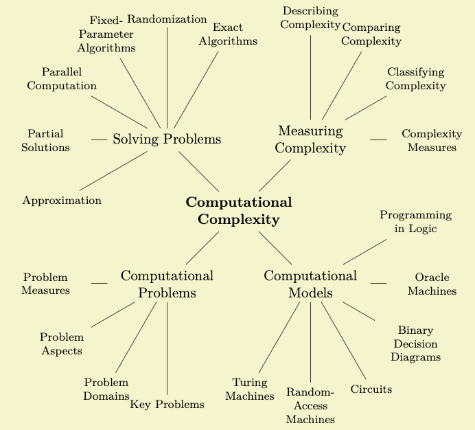
                \usetikzlibrary {trees}

                \tikz [text width=2.7cm, align=flush center,

                       grow cyclic,

                       level 1/.style={level distance=2.5cm,sibling angle=90},

                       level 2/.style={text width=2cm, font=\footnotesize, level distance=3cm,sibling angle=30}]

                  \node[font=\bfseries] {Computational
                Complexity} % root

                    child
                { node {Computational
                Problems}

                      child
                { node {Problem
                Measures} }

                      child
                { node {Problem
                Aspects} }

                      ... % as before
Johannes is pleased to learn that he can access and manipulate the nodes of the tree like any normal node. In particular, he can name them using the name= option or the (⟨name⟩) notation and he can use any available shape or style for the trees nodes. He can connect trees later on using the normal \draw (some node) -- (another node); syntax. In essence, the child command just computes an appropriate position for a node and adds a line from the child to the parent node.
6.3 Creating the Lecture Map
Johannes now has a first possible layout for his lecture map. The next step is to make it “look nicer”. For this, the mindmap library is helpful since it makes a number of styles available that will make a tree look like a nice “mind map” or “concept map”.
The first step is to include the mindmap library, which Johannes already did. Next, he must add one of the following options to a scope that will contain the lecture map: mindmap or large mindmap or huge mindmap. These options all have the same effect, except that for a large mindmap the predefined font size and node sizes are somewhat larger than for a standard mindmap and for a huge mindmap they are even larger. So, a large mindmap does not necessarily need to have a lot of concepts, but it will need a lot of paper.
The second step is to add the concept option to every node that will, indeed, be a concept of the mindmap. The idea is that some nodes of a tree will be real concepts, while other nodes might just be “simple children”. Typically, this is not the case, so you might consider saying every node/.style=concept.
The third step is to set up the sibling angle (rather than a sibling distance) to specify the angle between sibling concepts.
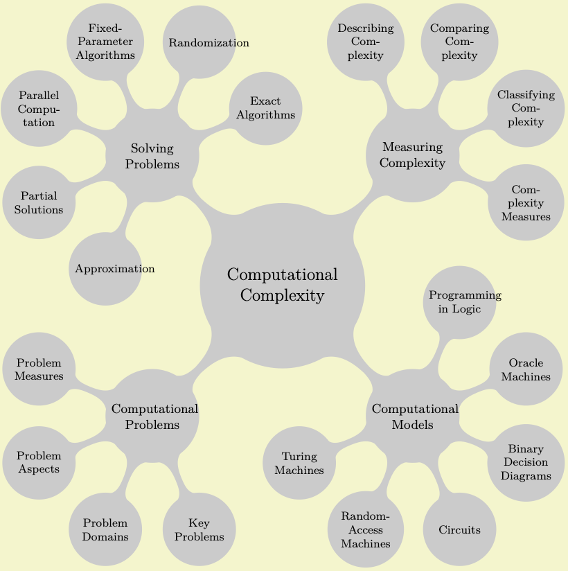
                \usetikzlibrary {mindmap}

                \tikz [mindmap, every node/.style=concept, concept color=black!20,

                       grow cyclic,

                       level 1/.append style={level distance=4.5cm,sibling angle=90},

                       level 2/.append style={level distance=3cm,sibling angle=45}]

                  \node [root concept] {Computational
                Complexity} % root

                    child
                { node {Computational
                Problems}

                      child
                { node {Problem
                Measures} }

                      child
                { node {Problem
                Aspects} }

                      ... % as before
When Johannes typesets the above map, TeX (rightfully) starts complaining about several overfull boxes and, indeed, words like “Randomization” stretch out beyond the circle of the concept. This seems a bit mysterious at first sight: Why does TeX not hyphenate the word? The reason is that TeX will never hyphenate the first word of a paragraph because it starts looking for “hyphenatable” letters only after a so-called glue. In order to have TeX hyphenate these single words, Johannes must use a bit of evil trickery: He inserts a \hskip0pt before the word. This has no effect except for inserting an (invisible) glue before the word and, thereby, allowing TeX to hyphenate the first word also. Since Johannes does not want to add \hskip0pt inside each node, he uses the execute at begin node option to make TikZ insert this text with every node.
                \usetikzlibrary {mindmap}

                \begin{tikzpicture}

                  [mindmap,

                   every node/.style={concept, execute at begin node=\hskip0pt},

                   concept color=black!20,

                   grow cyclic,

                   level 1/.append style={level distance=4.5cm,sibling angle=90},

                   level 2/.append style={level distance=3cm,sibling angle=45}]

                  \clip (-1,2) rectangle
                ++ (-4,5);

                  \node [root concept] {Computational
                Complexity} % root

                    child
                { node {Computational
                Problems}

                      child
                { node {Problem
                Measures} }

                      child
                { node {Problem
                Aspects} }

                      ... % as before

                \end{tikzpicture}
In the above example a clipping was used to show only part of the lecture map, in order to save space. The same will be done in the following examples, we return to the complete lecture map at the end of this tutorial.
Johannes is now eager to colorize the map. The idea is to use different colors for different parts of the map. He can then, during his lectures, talk about the “green” or the “red” topics. This will make it easier for his students to locate the topic he is talking about on the map. Since “computational problems” somehow sounds “problematic”, Johannes chooses red for them, while he picks green for the “solving problems”. The topics “measuring complexity” and “computational models” get more neutral colors; Johannes picks orange and blue.
To set the colors, Johannes must use the concept color option, rather than just, say, node [fill=red]. Setting just the fill color to red would, indeed, make the node red, but it would just make the node red and not the bar connecting the concept to its parent and also not its children. By comparison, the special concept color option will not only set the color of the node and its children, but it will also (magically) create appropriate shadings so that the color of a parent concept smoothly changes to the color of a child concept.
For the root concept Johannes decides to do something special: He sets the concept color to black, sets the line width to a large value, and sets the fill color to white. The effect of this is that the root concept will be encircled with a thick black line and the children are connected to the central concept via bars.
                \usetikzlibrary {mindmap}

                \begin{tikzpicture}

                  [mindmap,

                   every node/.style={concept, execute at begin node=\hskip0pt},

                   root concept/.append style={

                     concept color=black, fill=white, line width=1ex, text=black},

                   text=white,

                   grow cyclic,

                   level 1/.append style={level distance=4.5cm,sibling angle=90},

                   level 2/.append style={level distance=3cm,sibling angle=45}]

                   \clip (0,-1) rectangle
                ++(4,5);

                  \node [root concept] {Computational
                Complexity} % root

                    child
                [concept color=red] { node
                {Computational
                Problems}

                      child
                { node {Problem
                Measures} }

                      ... % as before

                    }

                    child
                [concept color=blue] { node
                {Computational
                Models}

                      child
                { node {Turing
                Machines} }

                      ... % as before

                    }

                    child
                [concept color=orange] { node
                {Measuring
                Complexity}

                      child
                { node {Complexity
                Measures} }

                      ... % as before

                    }

                    child
                [concept color=green!50!black] { node
                {Solving
                Problems}

                      child
                { node {Exact
                Algorithms} }

                      ... % as before

                    };

                \end{tikzpicture}
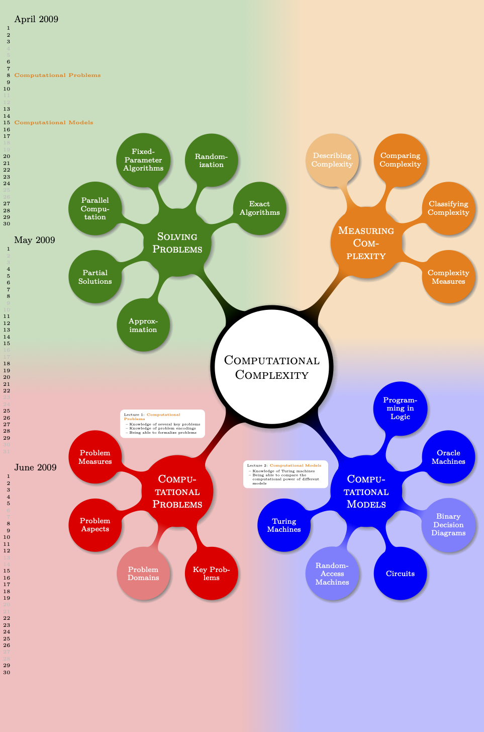
Johannes adds three finishing touches: First, he changes the font of the main concepts to small caps. Second, he decides that some concepts should be “faded”, namely those that are important in principle and belong on the map, but which he will not talk about in his lecture. To achieve this, Johannes defines four styles, one for each of the four main branches. These styles (a) set up the correct concept color for the whole branch and (b) define the faded style appropriately for this branch. Third, he adds a circular drop shadow, defined in the shadows library, to the concepts, just to make things look a bit more fancy.
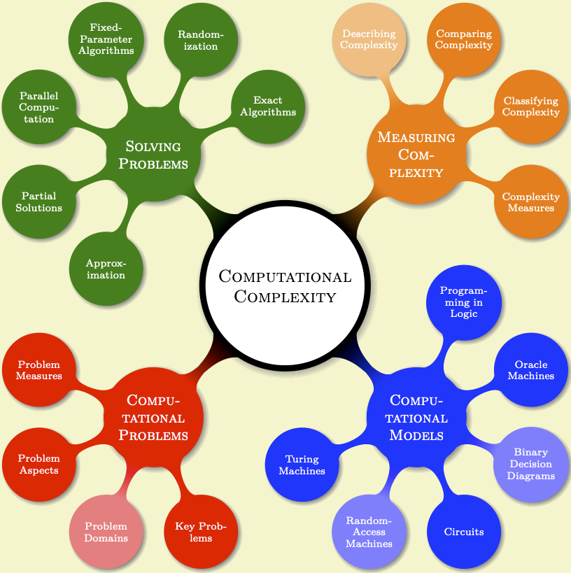
                \usetikzlibrary {mindmap,shadows}

                \begin{tikzpicture}[mindmap]

                  \begin{scope}[

                    every node/.style={concept, circular drop shadow,execute at begin node=\hskip0pt},

                    root concept/.append style={

                      concept color=black, fill=white, line width=1ex, text=black, font=\large\scshape},

                    text=white,

                    computational problems/.style={concept color=red,faded/.style={concept color=red!50}},

                    computational models/.style={concept color=blue,faded/.style={concept color=blue!50}},

                    measuring complexity/.style={concept color=orange,faded/.style={concept color=orange!50}},

                    solving problems/.style={concept color=green!50!black,faded/.style={concept color=green!50!black!50}},

                    grow cyclic,

                    level 1/.append style={level distance=4.5cm,sibling angle=90,font=\scshape},

                    level 2/.append style={level distance=3cm,sibling angle=45,font=\scriptsize}]

                    \node [root concept] {Computational
                Complexity} % root

                      child
                [computational problems] { node
                {Computational
                Problems}

                        child
                        { node
                {Problem
                Measures} }

                        child
                        { node
                {Problem
                Aspects} }

                        child
                [faded] { node
                {Problem
                Domains} }

                        child
                        { node
                {Key
                Problems} }

                      }

                      child
                [computational models] { node
                {Computational
                Models}

                        child
                        { node
                {Turing
                Machines} }

                        child
                [faded] { node
                {Random-Access
                Machines} }

                        ...

                  \end{scope}

                \end{tikzpicture}
6.4 Adding the Lecture Annotations
Johannes will give about a dozen lectures during the course “computational complexity”. For each lecture he has compiled a (short) list of learning targets that state what knowledge and qualifications his students should acquire during this particular lecture (note that learning targets are not the same as the contents of a lecture). For each lecture he intends to put a little rectangle on the map containing these learning targets and the name of the lecture, each time somewhere near the topic of the lecture. Such “little rectangles” are called “annotations” by the mindmap library.
In order to place the annotations next to the concepts, Johannes must assign names to the nodes of the concepts. He could rely on TikZ’s automatic naming of the nodes in a tree, where the children of a node named root are named root-1, root-2, root-3, and so on. However, since Johannes is not sure about the final order of the concepts in the tree, it seems better to explicitly name all concepts of the tree in the following manner:
                \node [root concept] (Computational Complexity) {Computational
                Complexity}

                  child [computational problems] { node
                (Computational Problems) {Computational
                Problems}

                    child
                        { node
                (Problem Measures) {Problem
                Measures} }

                    child
                        { node
                (Problem Aspects) {Problem
                Aspects} }

                    child
                [faded] { node
                (Problem Domains) {Problem
                Domains} }

                    child
                        { node
                (Key Problems) {Key
                Problems} }

                  }

                ...
The annotation style of the mindmap library mainly sets up a rectangular shape of appropriate size. Johannes configures the style by defining every annotation appropriately.
                \usetikzlibrary {mindmap,shadows}

                \begin{tikzpicture}[mindmap]

                  \clip (-5,-5) rectangle
                ++ (4,5);

                  \begin{scope}[

                     every node/.style={concept, circular drop shadow, ...}] % as before

                    \node [root concept] (Computational Complexity)    ...   % as before

                  \end{scope}


                  \begin{scope}[every annotation/.style={fill=black!40}]

                    \node [annotation, above] at
                (Computational Problems.north) {

                      Lecture
                1:
                Computational
                Problems

                      \begin{itemize}

                      \item Knowledge
                of
                several key
                problems

                      \item Knowledge
                of
                problem encodings

                      \item Being
                able
                to
                formalize
                problems

                      \end{itemize}

                    };

                  \end{scope}

                \end{tikzpicture}
Well, that does not yet look quite perfect. The spacing or the {itemize} is not really appropriate and the node is too large. Johannes can configure these things “by hand”, but it seems like a good idea to define a macro that will take care of these things for him. The “right” way to do this is to define a \lecture macro that takes a list of key–value pairs as argument and produces the desired annotation. However, to keep things simple, Johannes’ \lecture macro simply takes a fixed number of arguments having the following meaning: The first argument is the number of the lecture, the second is the name of the lecture, the third are positioning options like above, the fourth is the position where the node is placed, the fifth is the list of items to be shown, and the sixth is a date when the lecture will be held (this parameter is not yet needed, we will, however, need it later on).
                \def\lecture#1#2#3#4#5#6{

                  \node [annotation, #3, scale=0.65, text width=4cm, inner sep=2mm] at
                (#4) {

                    Lecture
                #1:
                \textcolor{orange}{\textbf{#2}}

                    \list{--}{\topsep=2pt\itemsep=0pt\parsep=0pt

                              \parskip=0pt\labelwidth=8pt\leftmargin=8pt

                              \itemindent=0pt\labelsep=2pt}

                    #5

                    \endlist

                  };

                }
                \usetikzlibrary {mindmap,shadows}

                \begin{tikzpicture}[mindmap,every annotation/.style={fill=white}]

                  \clip (-5,-5) rectangle
                ++ (4,5);

                  \begin{scope}[

                     every node/.style={concept, circular drop shadow, ... % as before


                    \node [root concept] (Computational Complexity) ... % as before


                  \end{scope}


                  \lecture{1}{Computational Problems}{above,xshift=-3mm}

                    {Computational Problems.north}{

                      \item Knowledge
                  of several key problems

                      \item Knowledge
                  of problem encodings

                      \item Being able
                  to formalize problems

                    }{2009-04-08}

                  \end{tikzpicture}
In the same fashion Johannes can now add the other lecture annotations. Obviously, Johannes will have some trouble fitting everything on a single A4-sized page, but by adjusting the spacing and some experimentation he can quickly arrange all the annotations as needed.
6.5 Adding the Background
Johannes has already used colors to organize his lecture map into four regions, each having a different color. In order to emphasize these regions even more strongly, he wishes to add a background coloring to each of these regions.
Adding these background colors turns out to be more tricky than Johannes would have thought. At first sight, what he needs is some sort of “color wheel” that is blue in the lower right direction and then changes smoothly to orange in the upper right direction and then to green in the upper left direction and so on. Unfortunately, there is no easy way of creating such a color wheel shading (although it can be done, in principle, but only at a very high cost, see section 69 for an example).
Johannes decides to do something a bit more basic: He creates four large rectangles, one for each of the four quadrants around the central concept, each colored with a light version of the quadrant. Then, in order to “smooth” the change between adjacent rectangles, he puts four shadings on top of them.
Since these background rectangles should go “behind” everything else, Johannes puts all his background stuff on the background layer.
In the following code, only the central concept is shown to save some space:

                \usetikzlibrary {backgrounds,mindmap,shadows}

                \begin{tikzpicture}[

                  mindmap,

                  concept color=black,

                  root concept/.append style={

                    concept,

                    circular drop shadow,

                    fill=white, line width=1ex,

                    text=black, font=\large\scshape}

                    ]


                  \clip (-1.5,-5) rectangle
                ++(4,10);


                  \node [root concept] (Computational Complexity) {Computational
                Complexity};


                  \begin{pgfonlayer}{background}

                    \clip (-1.5,-5) rectangle
                ++(4,10);


                    \colorlet{upperleft}{green!50!black!25}

                    \colorlet{upperright}{orange!25}

                    \colorlet{lowerleft}{red!25}

                    \colorlet{lowerright}{blue!25}


                     % The large rectangles:

                    \fill [upperleft]  (Computational Complexity) rectangle
                ++(-20,20);

                    \fill [upperright] (Computational Complexity) rectangle
                ++(20,20);

                    \fill [lowerleft]  (Computational Complexity) rectangle
                ++(-20,-20);

                    \fill [lowerright] (Computational Complexity) rectangle
                ++(20,-20);


                    % The shadings:

                    \shade [left color=upperleft,right color=upperright]

                      ([xshift=-1cm]Computational Complexity) rectangle
                ++(2,20);

                    \shade [left color=lowerleft,right color=lowerright]

                      ([xshift=-1cm]Computational Complexity) rectangle
                ++(2,-20);

                    \shade [top color=upperleft,bottom color=lowerleft]

                      ([yshift=-1cm]Computational Complexity) rectangle
                ++(-20,2);

                    \shade [top color=upperright,bottom color=lowerright]

                      ([yshift=-1cm]Computational Complexity) rectangle
                ++(20,2);

                  \end{pgfonlayer}

                \end{tikzpicture}
6.6 Adding the Calendar
Johannes intends to plan his lecture rather carefully. In particular, he already knows when each of his lectures will be held during the course. Naturally, this does not mean that Johannes will slavishly follow the plan and he might need longer for some subjects than he anticipated, but nevertheless he has a detailed plan of when which subject will be addressed.
Johannes intends to share this plan with his students by adding a calendar to the lecture map. In addition to serving as a reference on which particular day a certain topic will be addressed, the calendar is also useful to show the overall chronological order of the course.
In order to add a calendar to a TikZ graphic, the calendar library is most useful. The library provides the \calendar command, which takes a large number of options and which can be configured in many ways to produce just about any kind of calendar imaginable. For Johannes’ purposes, a simple day list downward will be a nice option since it produces a list of days that go “downward”.

                \usetikzlibrary {calendar}

                \tiny

                \begin{tikzpicture}

                  \calendar [day list downward,

                             name=cal,

                             dates=2009-04-01 to 2009-04-14]

                    if
                (weekend)

                      [black!25];

                \end{tikzpicture}
Using the name option, we gave a name to the calendar, which will allow us to reference the nodes that make up the individual days of the calendar later on. For instance, the rectangular node containing the 1 that represents April 1st, 2009, can be referenced as (cal-2009-04-01). The dates option is used to specify an interval for which the calendar should be drawn. Johannes will need several months in his calendar, but the above example only shows two weeks to save some space.
Note the if (weekend) construct. The \calendar command is followed by options and then by if-statements. These if-statements are checked for each day of the calendar and when a date passes this test, the options or the code following the if-statement is executed. In the above example, we make weekend days (Saturdays and Sundays, to be precise) lighter than normal days. (Use your favorite calendar to check that, indeed, April 5th, 2009, is a Sunday.)
As mentioned above, Johannes can reference the nodes that are used to typeset days. Recall that his \lecture macro already got passed a date, which we did not use, yet. We can now use it to place the lecture’s title next to the date when the lecture will be held:
                \def\lecture#1#2#3#4#5#6{

                  % As before:

                  \node [annotation, #3, scale=0.65, text width=4cm, inner sep=2mm] at
                (#4) {

                    Lecture
                #1:
                \textcolor{orange}{\textbf{#2}}

                    \list{--}{\topsep=2pt\itemsep=0pt\parsep=0pt

                              \parskip=0pt\labelwidth=8pt\leftmargin=8pt

                              \itemindent=0pt\labelsep=2pt}

                    #5

                    \endlist

                  };

                  % New:

                  \node [anchor=base west] at
                (cal-#6.base east) {\textcolor{orange}{\textbf{#2}}};

                }
Johannes can now use this new \lecture command as follows (in the example, only the new part of the definition is used):

                \usetikzlibrary {calendar}

                \tiny

                \begin{tikzpicture}

                  \calendar [day list downward,

                             name=cal,

                             dates=2009-04-01 to 2009-04-14]

                    if
                (weekend)

                      [black!25];


                  % As before:

                  \lecture{1}{Computational
                Problems}{above,xshift=-3mm}

                  {Computational
                Problems.north}{

                    \item Knowledge
                of
                several key
                problems

                    \item Knowledge
                of
                problem encodings

                    \item Being
                able
                to
                formalize
                problems

                  }{2009-04-08}

                \end{tikzpicture}
As a final step, Johannes needs to add a few more options to the calendar command: He uses the month text option to configure how the text of a month is rendered (see Section 47 for details) and then typesets the month text at a special position at the beginning of each month.
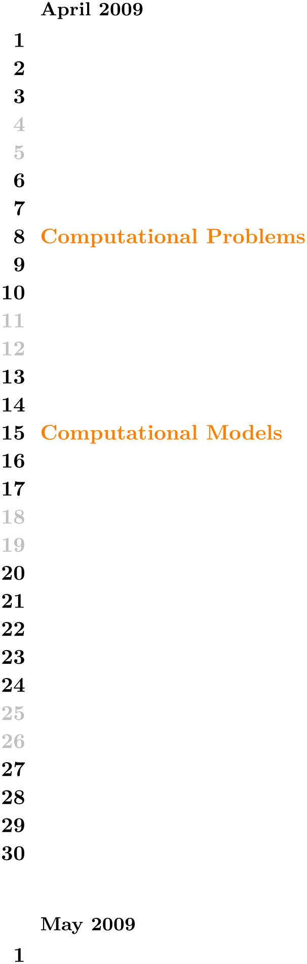
                \usetikzlibrary {calendar}

                \tiny

                \begin{tikzpicture}

                  \calendar [day list downward,

                             month text=\%mt\ \%y0,

                             month yshift=3.5em,

                             name=cal,

                             dates=2009-04-01 to 2009-05-01]

                    if
                (weekend)

                      [black!25]

                    if
                (day of month=1) {

                      \node at
                (0pt,1.5em) [anchor=base west] {\small\tikzmonthtext};

                    };


                  \lecture{1}{Computational
                Problems}{above,xshift=-3mm}

                  {Computational
                Problems.north}{

                    \item Knowledge
                of
                several key
                problems

                    \item Knowledge
                of
                problem encodings

                    \item Being
                able
                to
                formalize
                problems

                  }{2009-04-08}


                  \lecture{2}{Computational
                Models}{above,xshift=-3mm}

                  {Computational
                Models.north}{

                    \item Knowledge
                of
                Turing machines

                    \item Being
                able
                to
                compare the
                computational
                power
                of
                different

                      models

                  }{2009-04-15}

                \end{tikzpicture}
6.7 The Complete Code
Putting it all together, Johannes gets the following code:
First comes the definition of the \lecture command:
                \def\lecture#1#2#3#4#5#6{

                  % As before:

                  \node [annotation, #3, scale=0.65, text width=4cm, inner sep=2mm, fill=white] at
                (#4) {

                    Lecture
                #1:
                \textcolor{orange}{\textbf{#2}}

                    \list{--}{\topsep=2pt\itemsep=0pt\parsep=0pt

                              \parskip=0pt\labelwidth=8pt\leftmargin=8pt

                              \itemindent=0pt\labelsep=2pt}

                    #5

                    \endlist

                  };

                  % New:

                  \node [anchor=base west] at
                (cal-#6.base east) {\textcolor{orange}{\textbf{#2}}};

                }
This is followed by the main mindmap setup…
                \noindent

                \begin{tikzpicture}

                  \begin{scope}[

                    mindmap,

                    every node/.style={concept, circular drop shadow,execute at begin node=\hskip0pt},

                    root concept/.append style={

                      concept color=black,

                      fill=white, line width=1ex,

                      text=black, font=\large\scshape},

                    text=white,

                    computational problems/.style={concept color=red,faded/.style={concept color=red!50}},

                    computational models/.style={concept color=blue,faded/.style={concept color=blue!50}},

                    measuring complexity/.style={concept color=orange,faded/.style={concept color=orange!50}},

                    solving problems/.style={concept color=green!50!black,faded/.style={concept color=green!50!black!50}},

                    grow cyclic,

                    level 1/.append style={level distance=4.5cm,sibling angle=90,font=\scshape},

                    level 2/.append style={level distance=3cm,sibling angle=45,font=\scriptsize}]
…and contents:
                  \node [root concept] (Computational Complexity) {Computational
                Complexity} % root

                      child
                [computational problems] { node
                [yshift=-1cm] (Computational Problems) {Computational
                Problems}

                        child
                        { node
                (Problem Measures) {Problem
                Measures} }

                        child
                        { node
                (Problem Aspects) {Problem
                Aspects} }

                        child
                [faded] { node
                (problem Domains) {Problem
                Domains} }

                        child
                        { node
                (Key Problems) {Key
                Problems} }

                      }

                      child
                [computational models] { node
                [yshift=-1cm]  (Computational Models) {Computational
                Models}

                        child
                        { node
                (Turing Machines) {Turing
                Machines} }

                        child
                [faded] { node
                (Random-Access Machines) {Random-Access
                Machines} }

                        child
                        { node
                (Circuits) {Circuits} }

                        child
                [faded] { node
                (Binary Decision Diagrams) {Binary
                Decision
                Diagrams} }

                        child
                        { node
                (Oracle Machines) {Oracle
                Machines} }

                        child
                        { node
                (Programming in Logic) {Programming
                in
                Logic} }

                      }

                      child
                [measuring complexity] { node
                [yshift=1cm] (Measuring Complexity) {Measuring
                Complexity}

                        child
                        { node
                (Complexity Measures) {Complexity
                Measures} }

                        child
                        { node
                (Classifying Complexity) {Classifying
                Complexity} }

                        child
                        { node
                (Comparing Complexity) {Comparing
                Complexity} }

                        child
                [faded] { node
                (Describing Complexity) {Describing
                Complexity} }

                      }

                      child
                [solving problems] { node
                [yshift=1cm] (Solving Problems) {Solving
                Problems}

                        child
                        { node
                (Exact Algorithms) {Exact
                Algorithms} }

                        child
                        { node
                (Randomization) {Randomization} }

                        child
                        { node
                (Fixed-Parameter Algorithms) {Fixed-Parameter
                Algorithms} }

                        child
                        { node
                (Parallel Computation) {Parallel
                Computation} }

                        child
                        { node
                (Partial Solutions) {Partial
                Solutions} }

                        child
                        { node
                (Approximation) {Approximation} }

                      };

                  \end{scope}
Now comes the calendar code:
The lecture annotations:
                  \lecture{1}{Computational
                Problems}{above,xshift=-5mm,yshift=5mm}{Computational
                Problems.north}{

                    \item Knowledge
                of
                several key
                problems

                    \item Knowledge
                of
                problem encodings

                    \item Being
                able
                to
                formalize
                problems

                  }{2009-04-08}


                  \lecture{2}{Computational
                Models}{above
                left}

                  {Computational
                Models.west}{

                    \item Knowledge
                of
                Turing machines

                    \item Being
                able
                to
                compare the
                computational
                power
                of
                different

                      models

                  }{2009-04-15}
Finally, the background:
                  \begin{pgfonlayer}{background}

                    \clip[xshift=-1cm] (-.5\textwidth,-.5\textheight) rectangle
                ++(\textwidth,\textheight);


                    \colorlet{upperleft}{green!50!black!25}

                    \colorlet{upperright}{orange!25}

                    \colorlet{lowerleft}{red!25}

                    \colorlet{lowerright}{blue!25}


                     % The large rectangles:

                    \fill [upperleft]  (Computational Complexity) rectangle
                ++(-20,20);

                    \fill [upperright] (Computational Complexity) rectangle
                ++(20,20);

                    \fill [lowerleft]  (Computational Complexity) rectangle
                ++(-20,-20);

                    \fill [lowerright] (Computational Complexity) rectangle
                ++(20,-20);


                    % The shadings:

                    \shade [left color=upperleft,right color=upperright]

                      ([xshift=-1cm]Computational Complexity) rectangle
                ++(2,20);

                    \shade [left color=lowerleft,right color=lowerright]

                      ([xshift=-1cm]Computational Complexity) rectangle
                ++(2,-20);

                    \shade [top color=upperleft,bottom color=lowerleft]

                      ([yshift=-1cm]Computational Complexity) rectangle
                ++(-20,2);

                    \shade [top color=upperright,bottom color=lowerright]

                      ([yshift=-1cm]Computational Complexity) rectangle
                ++(20,2);

                  \end{pgfonlayer}

                \end{tikzpicture}
The next page shows the resulting lecture map in all its glory (it would be somewhat more glorious, if there were more lecture annotations, but you should get the idea).