TikZ and PGF Manual
The Basic Layer
108 Coordinate, Canvas, and Nonlinear Transformations
108.1 Overview
pgf offers different ways of scaling, shifting, and rotating (these operations are generally known as transformations) graphics: You can apply coordinate transformations to all coordinates, you can apply canvas transformations to the canvas on which you draw, and you can apply additional nonlinear transformations. (The names “coordinate” and “canvas” transformations are not standard, I introduce them only for the purposes of this manual.)
The differences are the following:
-
• As the name “coordinate transformation” suggests, coordinate transformations apply only to coordinates. For example, when you specify a coordinate like \pgfpoint{1cm}{2cm} and you wish to “use” this coordinate – for example as an argument to a \pgfpathmoveto command – then the coordinate transformation matrix is applied to the coordinate, resulting in a new coordinate. Continuing the example, if the current coordinate transformation is “scale by a factor of two”, the coordinate \pgfpoint{1cm}{2cm} actually designates the point \((2\mathrm {cm},4\mathrm {cm})\).
Note that coordinate transformations apply only to coordinates. They do not apply to, say, line width or shadings or text.
-
• The effect of a “canvas transformation” like “scale by a factor of two” can be imagined as follows: You first draw your picture on a “rubber canvas” normally. Then, once you are done, the whole canvas is transformed, in this case stretched by a factor of two. In the resulting image everything will be larger: Text, lines, coordinates, and shadings.
-
• Nonlinear transformations are a special form of coordinate transformations that are, as the name suggests, not linear. The support for nonlinear transformations is quite different from the support for linear coordinate transformations, the main reason being speed: While linear coordinate transformations can be applied very quickly (pgf does so almost constantly), nonlinear transformations are much harder to apply and also to use. For this reason, nonlinear transformations are implemented in a special module nonlineartransformations that has to be loaded explicitly. By default, they are not available.
In many cases, it is preferable that you use coordinate transformations and not canvas transformations. When canvas transformations are used, pgf looses track of the coordinates of nodes and shapes. Also, canvas transformations often cause undesirable effects like changing text size. For these reasons, pgf makes it easy to setup the coordinate transformation, but a bit harder to change the canvas transformation. Because of the speed penalties caused by nonlinear transformations, they are even harder to set up.
108.2 Coordinate Transformations
108.2.1 How PGF Keeps Track of the Coordinate Transformation Matrix
pgf has an internal coordinate transformation matrix. This matrix is applied to coordinates “in certain situations”. This means that the matrix is not always applied to every coordinate “no matter what”. Rather, pgf tries to be reasonably smart at when and how this matrix should be applied. The most prominent examples are the path construction commands, which apply the coordinate transformation matrix to their inputs.
The coordinate transformation matrix consists of four numbers \(a\), \(b\), \(c\), and \(d\), and two dimensions \(s\) and \(t\). When the coordinate transformation matrix is applied to a coordinate \((x,y)\), the new coordinate \((ax+cy+s,bx+dy+t)\) results. For more details on how transformation matrices work in general, please see, for example, the pdf or PostScript reference or a textbook on computer graphics.
The coordinate transformation matrix is equal to the identity matrix at the beginning. More precisely, \(a=1\), \(b=0\), \(c=0\), \(d=1\), \(s=0\mathrm {pt}\), and \(t=0\mathrm {pt}\).
The different coordinate transformation commands will modify the matrix by concatenating it with another transformation matrix. This way the effect of applying several transformation commands will accumulate.
The coordinate transformation matrix is local to the current TeX group (unlike the canvas transformation matrix, which is local to the current {pgfscope}). Thus, the effect of adding a coordinate transformation to the coordinate transformation matrix will last only till the end of the current TeX group.
108.2.2 Commands for Relative Coordinate Transformations
The following commands add a basic coordinate transformation to the current coordinate transformation matrix. For all commands, the transformation is applied in addition to any previous coordinate transformations.
-
\pgftransformshift{⟨point⟩} 
Shifts coordinates by ⟨point⟩.
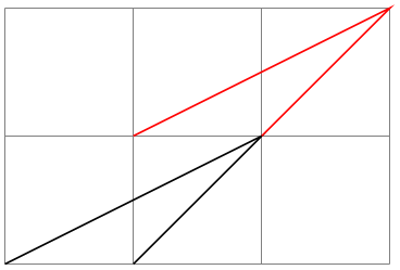
                    \begin{tikzpicture}

                      \draw[help lines] (0,0) grid
                    (3,2);

                      \draw      (0,0) --
                    (2,1) --
                    (1,0);

                      \pgftransformshift{\pgfpoint{1cm}{1cm}}

                      \draw[red] (0,0) --
                    (2,1) --
                    (1,0);

                    \end{tikzpicture}
-
\pgftransformxshift{⟨dimensions⟩} 
Shifts coordinates by ⟨dimension⟩ along the \(x\)-axis.

                    \begin{tikzpicture}

                      \draw[help lines] (0,0) grid
                    (3,2);

                      \draw      (0,0) --
                    (2,1) --
                    (1,0);

                      \pgftransformxshift{.5cm}

                      \draw[red] (0,0) --
                    (2,1) --
                    (1,0);

                    \end{tikzpicture}
-
\pgftransformyshift{⟨dimensions⟩} 
Like \pgftransformxshift, only for the \(y\)-axis.
-
\pgftransformscale{⟨factor⟩} 
Scales coordinates by ⟨factor⟩.
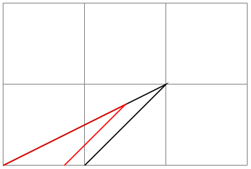
                    \begin{tikzpicture}

                      \draw[help lines] (0,0) grid
                    (3,2);

                      \draw      (0,0) --
                    (2,1) --
                    (1,0);

                      \pgftransformscale{.75}

                      \draw[red] (0,0) --
                    (2,1) --
                    (1,0);

                    \end{tikzpicture}
-
\pgftransformxscale{⟨factor⟩} 
Scales coordinates by ⟨factor⟩ in the \(x\)-direction.
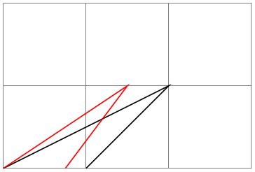
                    \begin{tikzpicture}

                      \draw[help lines] (0,0) grid
                    (3,2);

                      \draw      (0,0) --
                    (2,1) --
                    (1,0);

                      \pgftransformxscale{.75}

                      \draw[red] (0,0) --
                    (2,1) --
                    (1,0);

                    \end{tikzpicture}
-
\pgftransformyscale{⟨factor⟩} 
Like \pgftransformxscale, only for the \(y\)-axis.
-
\pgftransformxslant{⟨factor⟩} 
Slants coordinates by ⟨factor⟩ in the \(x\)-direction. Here, a factor of 1 means \(45^\circ \).

                    \begin{tikzpicture}

                      \draw[help lines] (0,0) grid
                    (3,2);

                      \draw      (0,0) --
                    (2,1) --
                    (1,0);

                      \pgftransformxslant{.5}

                      \draw[red] (0,0) --
                    (2,1) --
                    (1,0);

                    \end{tikzpicture}
-
\pgftransformyslant{⟨factor⟩} 
Slants coordinates by ⟨factor⟩ in the \(y\)-direction.
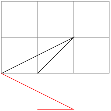
                    \begin{tikzpicture}

                      \draw[help lines] (0,0) grid
                    (3,2);

                      \draw      (0,0) --
                    (2,1) --
                    (1,0);

                      \pgftransformyslant{-1}

                      \draw[red] (0,0) --
                    (2,1) --
                    (1,0);

                    \end{tikzpicture}
-
\pgftransformrotate{⟨angles⟩} 
Rotates coordinates counterclockwise by ⟨angles⟩ given in degrees.
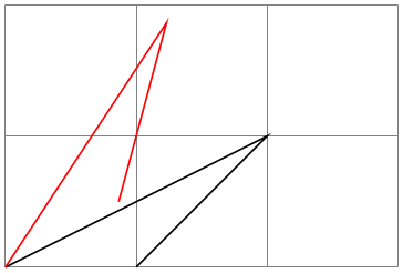
                    \begin{tikzpicture}

                      \draw[help lines] (0,0) grid
                    (3,2);

                      \draw      (0,0) --
                    (2,1) --
                    (1,0);

                      \pgftransformrotate{30}

                      \draw[red] (0,0) --
                    (2,1) --
                    (1,0);

                    \end{tikzpicture}
-
\pgftransformtriangle{⟨a⟩}{⟨b⟩}{⟨c⟩} 
This command transforms the coordinate system in such a way that the triangle given by the points ⟨a⟩, ⟨b⟩ and ⟨c⟩ lies at the coordinates \((0,0)\), \((1\mathrm {pt},0\mathrm {pt})\) and \((0\mathrm {pt},1\mathrm {pt})\).
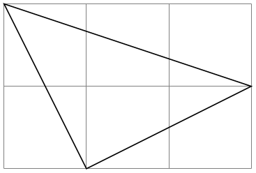
                    \begin{tikzpicture}

                      \draw[help lines] (0,0) grid
                    (3,2);

                      \pgftransformtriangle

                      {\pgfpoint{1cm}{0cm}}

                      {\pgfpoint{0cm}{2cm}}

                      {\pgfpoint{3cm}{1cm}}


                      \draw (0,0) --
                    (1pt,0pt) --
                    (0pt,1pt) --
                    cycle;

                    \end{tikzpicture}
-
\pgftransformcm{⟨a⟩}{⟨b⟩}{⟨c⟩}{⟨d⟩}{⟨point⟩} 
Applies the transformation matrix given by \(a\), \(b\), \(c\), and \(d\) and the shift ⟨point⟩ to coordinates (in addition to any previous transformations already in force).
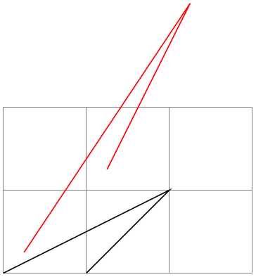
                    \begin{tikzpicture}

                      \draw[help lines] (0,0) grid
                    (3,2);

                      \draw      (0,0) --
                    (2,1) --
                    (1,0);

                      \pgftransformcm{1}{1}{0}{1}{\pgfpoint{.25cm}{.25cm}}

                      \draw[red] (0,0) --
                    (2,1) --
                    (1,0);

                    \end{tikzpicture}
-
\pgftransformarrow{⟨start⟩}{⟨end⟩} 
Shifts coordinates to the end of the line going from ⟨start⟩ to ⟨end⟩ with the correct rotation.
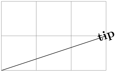
                    \begin{tikzpicture}

                      \draw[help lines] (0,0) grid
                    (3,2);

                      \draw      (0,0) --
                    (3,1);

                      \pgftransformarrow{\pgfpointorigin}{\pgfpoint{3cm}{1cm}}

                      \pgftext{tip}

                    \end{tikzpicture}
-
\pgftransformlineattime{⟨time⟩}{⟨start⟩}{⟨end⟩} 
Shifts coordinates by a specific point on a line at a specific time. The point by which the coordinate is shifted is calculated by calling \pgfpointlineattime, see Section 101.5.2.
In addition to shifting the coordinate, a rotation may also be applied. Whether this is the case depends on whether the TeX if \ifpgfslopedattime is set to true or not.

                    \begin{tikzpicture}

                      \draw[help lines] (0,0) grid
                    (3,2);

                      \draw      (0,0) --
                    (2,1);

                      \pgftransformlineattime{.25}{\pgfpointorigin}{\pgfpoint{2cm}{1cm}}

                      \pgftext{Hi!}

                    \end{tikzpicture}

                    \begin{tikzpicture}

                      \draw[help lines] (0,0) grid
                    (3,2);

                      \draw      (0,0) --
                    (2,1);

                      \pgfslopedattimetrue

                      \pgftransformlineattime{.25}{\pgfpointorigin}{\pgfpoint{2cm}{1cm}}

                      \pgftext{Hi!}

                    \end{tikzpicture}
If \ifpgfslopedattime is true, another TeX \if is important: \ifpgfallowupsidedowattime. If this is false, pgf will ensure that the rotation is done in such a way that text is never “upside down”.
There is another TeX \if that influences this command. If you set \ifpgfresetnontranslationattime to true, then, between shifting the coordinate and (possibly) rotating/sloping the coordinate, the command \pgftransformresetnontranslations is called. See the description of this command for details.
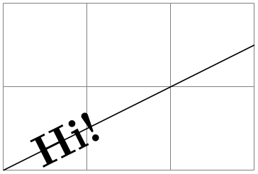
                    \begin{tikzpicture}

                      \draw[help lines] (0,0) grid
                    (3,2);

                      \pgftransformscale{1.5}

                      \draw      (0,0) --
                    (2,1);

                      \pgfslopedattimetrue

                      \pgfresetnontranslationattimefalse

                      \pgftransformlineattime{.25}{\pgfpointorigin}{\pgfpoint{2cm}{1cm}}

                      \pgftext{Hi!}

                    \end{tikzpicture}
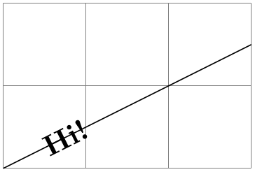
                    \begin{tikzpicture}

                      \draw[help lines] (0,0) grid
                    (3,2);

                      \pgftransformscale{1.5}

                      \draw      (0,0) --
                    (2,1);

                      \pgfslopedattimetrue

                      \pgfresetnontranslationattimetrue

                      \pgftransformlineattime{.25}{\pgfpointorigin}{\pgfpoint{2cm}{1cm}}

                      \pgftext{Hi!}

                    \end{tikzpicture}
-
\pgftransformcurveattime{⟨time⟩}{⟨start⟩}{⟨first support⟩}{⟨second support⟩}{⟨end⟩} 
Shifts coordinates by a specific point on a curve at a specific time, see Section 101.5.2 once more.
As for the line-at-time transformation command, \ifpgfslopedattime decides whether an additional rotation should be applied. Again, the value of \ifpgfallowupsidedowattime is also considered.
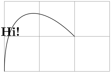
                    \begin{tikzpicture}

                      \draw[help lines] (0,0) grid
                    (3,2);

                      \draw      (0,0) .. controls
                    (0,2) and
                    (1,2) .. (2,1);

                      \pgftransformcurveattime{.25}{\pgfpointorigin}

                        {\pgfpoint{0cm}{2cm}}{\pgfpoint{1cm}{2cm}}{\pgfpoint{2cm}{1cm}}

                      \pgftext{Hi!}

                    \end{tikzpicture}
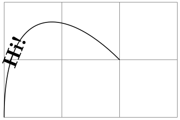
                    \begin{tikzpicture}

                      \draw[help lines] (0,0) grid
                    (3,2);

                      \draw      (0,0) .. controls
                    (0,2) and
                    (1,2) .. (2,1);

                      \pgfslopedattimetrue

                      \pgftransformcurveattime{.25}{\pgfpointorigin}

                        {\pgfpoint{0cm}{2cm}}{\pgfpoint{1cm}{2cm}}{\pgfpoint{2cm}{1cm}}

                      \pgftext{Hi!}

                    \end{tikzpicture}
The value of \ifpgfresetnontranslationsattime is also taken into account.
-
\pgftransformarcaxesattime{⟨time \(t\)⟩}{⟨center⟩}{⟨0-degree axis⟩}{⟨90-degree axis⟩}{⟨start angle⟩}{⟨end angle⟩} 
Shifts coordinates by a specific point on an arc at a specific time, see Section 101.5.2 once more.
As for the previous commands, \ifpgfslopedattime decides whether an additional rotation should be applied and \ifpgfallowupsidedowattime is also considered.
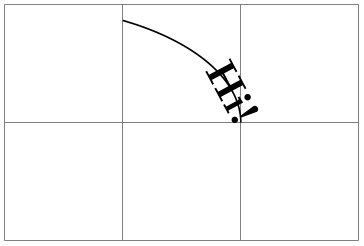
                    \begin{tikzpicture}

                      \draw[help lines] (0,0) grid
                    (3,2);

                      \pgfpathmoveto{\pgfpoint{2cm}{1cm}}

                      \pgfpatharcaxes{0}{60}{\pgfpoint{2cm}{0cm}}{\pgfpoint{0cm}{1cm}}

                      \pgfusepath{stroke}

                      \pgfslopedattimetrue

                      \pgftransformarcaxesattime{.25}

                        {\pgfpoint{0cm}{1cm}}

                        {\pgfpoint{2cm}{0cm}}{\pgfpoint{0cm}{1cm}}

                        {0}{60}

                      \pgftext{Hi!}

                    \end{tikzpicture}
The value of \ifpgfresetnontranslationsattime is also taken into account.
-
\ifpgfslopedattime 
Decides whether the “at time” transformation commands also rotate coordinates or not.
-
\ifpgfallowupsidedowattime 
Decides whether the “at time” transformation commands should allow the rotation be done in such a way that “upside-down text” can result.
-
\ifpgfresetnontranslationsattime 
Decides whether the “at time” transformation commands should reset the non-translations between shifting and rotating.
108.2.3 Commands for Absolute Coordinate Transformations
The coordinate transformation commands introduced up to now are always applied in addition to any previous transformations. In contrast, the commands presented in the following can be used to change the transformation matrix “in absolute terms”. Note that this is, in general, dangerous and will often produce unexpected effects. You should use these commands only if you really know what you are doing.
-
\pgftransformreset 
Resets the coordinate transformation matrix to the identity matrix. Thus, once this command is given no transformations are applied till the end of the scope.
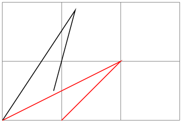
                    \begin{tikzpicture}

                      \draw[help lines] (0,0) grid
                    (3,2);

                      \pgftransformrotate{30}

                      \draw      (0,0) --
                    (2,1) --
                    (1,0);

                      \pgftransformreset

                      \draw[red] (0,0) --
                    (2,1) --
                    (1,0);

                    \end{tikzpicture}
-
\pgftransformresetnontranslations 
This command sets the \(a\), \(b\), \(c\), and \(d\) part of the coordinate transformation matrix to \(a=1\), \(b=0\), \(c=0\), and \(d=1\). However, the current shifting of the matrix is not modified.
The effect of this command is that any rotation/scaling/slanting is undone in the current TeX group, but the origin is not “moved back”.
This command is mostly useful directly before a \pgftext command to ensure that the text is not scaled or rotated.
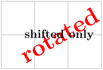
                    \begin{tikzpicture}

                      \draw[help lines] (0,0) grid
                    (3,2);

                      \pgftransformscale{2}

                      \pgftransformrotate{30}

                      \pgftransformxshift{1cm}

                      {\color{red}\pgftext{rotated}}

                      \pgftransformresetnontranslations

                      \pgftext{shifted
                    only}

                    \end{tikzpicture}
-
\pgftransforminvert 
Replaces the coordinate transformation matrix by a coordinate transformation matrix that “exactly undoes the original transformation”. For example, if the original transformation was “scale by 2 and then shift right by 1cm” the new one is “shift left by 1cm and then scale by \(1/2\)”.
This command will produce an error if the determinant of the matrix is too small, that is, if the matrix is near-singular.
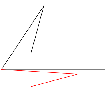
                    \begin{tikzpicture}

                      \draw[help lines] (0,0) grid
                    (3,2);

                      \pgftransformrotate{30}

                      \draw      (0,0) --
                    (2,1) --
                    (1,0);

                      \pgftransforminvert

                      \draw[red] (0,0) --
                    (2,1) --
                    (1,0);

                    \end{tikzpicture}
108.2.4 Saving and Restoring the Coordinate Transformation Matrix
There are two commands for saving and restoring coordinate transformation matrices.
-
\pgfgettransform{⟨macro⟩} 
This command will (locally) define ⟨macro⟩ to a representation of the current coordinate transformation matrix. This matrix can later on be reinstalled using \pgfsettransform.
-
\pgfsettransform{⟨macro⟩} 
Reinstalls a coordinate transformation matrix that was previously saved using \pgfgettransform.
-
\pgfgettransformentries{⟨macro for a⟩}{⟨macro for b⟩}{⟨macro for c⟩}{⟨macro for d⟩}{⟨macro for shift x⟩}{⟨macro for shift y⟩} 
This command is similar to \pgfgettransform except that it stores the current coordinate transformation matrix in a set of six macros.
The matrix can later on be reinstalled using \pgfsettransformentries. Furthermore, all these macros (or just a few of them) can be used as arguments for \pgftransformcm.
-
\pgfsettransformentries{⟨a⟩}{⟨b⟩}{⟨c⟩}{⟨d⟩}{⟨shiftx⟩}{⟨shifty⟩} 
Reinstalls a coordinate transformation matrix that was previously saved using the storage command \pgfgettransformentries. This command can also be used to replace any previously existing coordinate transformation matrix (it is thus equivalent to \pgftransformreset followed by \pgftransformcm).
108.2.5 Applying Coordinate Transformation to Points
-
\pgfpointtransformed{⟨point⟩} 
Applies current transformation matrix to {⟨point⟩} \((x,y)\) and returns a transformed point \((ax+cy+s,bx+dy+t)\). Normally, this is done automatically by commands like \pgfpathlineto or \pgfpathmoveto, but sometimes you may wish to access a transformed point yourself.
108.2.6 Computing Adjustments for Coordinate Transformations
-
\pgftransformationadjustments 
-
\pgfhorizontaltransformationadjustment 
-
\pgfverticaltransformationadjustment 
This command computes “adjustments” for the current transformation matrix so that even when you install a transformation matrix that scales everything by a certain factor, you can still draw something of “an absolute size”. Suppose for instance that you install a transformation matrix that scales everything by a factor of 4 and you now wish to draw a horizontal line of length 1cm. Then, if you do not reset the transformation matrix, you can draw a line of logical length 2.5mm, which will then get scaled to a line of 1cm. Things get more difficult in case you scale things only, say, vertically. In this case, the adjustment necessary for horizontal lines is different from the one needed for vertical lines.
This function computes two scaling factors, one for horizontal lines and one for vertical lines, and stores them in the following macros:
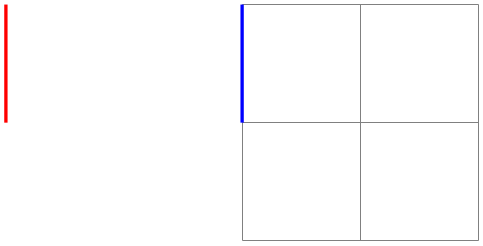
When you scale the length of a horizontal line by this factor in the current transformation, you compensate for the scaling. Formally, it is \(1/\|\mathit {transform}(1,0)\|_2\), where \(\mathit {transform}\) applies the current transformations matrix to the given number.

                        \begin{tikzpicture}

                          \draw [help lines] (0,0) grid
                        (2,2);

                          \begin{scope}[xscale=2,thick]

                            \draw [red] (1,1) --
                        ++(1,0);


                            \pgftransformationadjustments

                            \draw [blue] (1,0) --
                        ++(\pgfhorizontaltransformationadjustment,0);

                          \end{scope}

                        \end{tikzpicture}
                        \begin{tikzpicture}

                          \draw [help lines] (0,0) grid
                        (2,2);

                          \begin{scope}[xscale=2,thick,rotate=90]

                            \draw [red] (1,1) --
                        ++(1,0);


                            \pgftransformationadjustments

                            \draw [blue] (1,0) --
                        ++(\pgfhorizontaltransformationadjustment,0);

                          \end{scope}

                        \end{tikzpicture}
\(1/\|\mathit {transform}(0,1)\|_2\).
Note that the “right” way to draw a line of absolute length 1cm in a transformed coordinate system is to first compute the start point and to then reset the transformation matrix. The transformation adjustments computed here are important only in situations where you cannot do this, for instance when an outer xsep must be set.
108.3 Canvas Transformations
The canvas transformation matrix is not managed by pgf, but by the output format like pdf or PostScript. All that pgf does is to call appropriate low-level \pgfsys@ commands to change the canvas transformation matrix.
Unlike coordinate transformations, canvas transformations apply to “everything”, including images, text, shadings, line thickness, and so on. The idea is that a canvas transformation really stretches and deforms the canvas after the graphic is finished.
Unlike coordinate transformations, canvas transformations are local to the current {pgfscope}, not to the current TeX group. This is due to the fact that they are managed by the backend driver, not by TeX or pgf.
Unlike the coordinate transformation matrix, it is not possible to “reset” the canvas transformation matrix. The only way to change it is to concatenate it with another canvas transformation matrix or to end the current {pgfscope}.
Unlike coordinate transformations, pgf does not “keep track” of canvas transformations. In particular, it will not be able to correctly save the coordinates of shapes or nodes when a canvas transformation is used.
108.3.1 Applying General Canvas Transformations
pgf does not offer many commands for modifying the canvas transformation matrix. Instead, different commands allow you to concatenate the canvas transformation matrix with a coordinate transformation matrix (and there are numerous commands for specifying a coordinate transformation, see the previous section).
-
\pgflowlevelsynccm 
This command concatenates the canvas transformation matrix with the current coordinate transformation matrix. Afterward, the coordinate transformation matrix is reset.
The effect of this command is to “synchronize” the coordinate transformation matrix and the canvas transformation matrix. All transformations that were previously applied by the coordinate transformations matrix are now applied by the canvas transformation matrix.
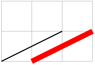
                    \begin{tikzpicture}

                      \draw[help lines] (0,0) grid
                    (3,2);

                      \pgfsetlinewidth{1pt}

                      \pgftransformscale{5}

                      \draw      (0,0) --
                    (0.4,.2);

                      \pgftransformxshift{0.2cm}

                      \pgflowlevelsynccm

                      \draw[red] (0,0) --
                    (0.4,.2);

                    \end{tikzpicture}
-
\pgflowlevel{⟨transformation code⟩} 
This command concatenates the canvas transformation matrix with the coordinate transformation specified by ⟨transformation code⟩.
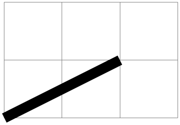
                    \begin{tikzpicture}

                      \draw[help lines] (0,0) grid
                    (3,2);

                      \pgfsetlinewidth{1pt}

                      \pgflowlevel{\pgftransformscale{5}}

                      \draw      (0,0) --
                    (0.4,.2);

                    \end{tikzpicture}
-
\pgflowlevelobj{⟨transformation code⟩}{⟨code⟩} 
This command creates a local {pgfscope}. Inside this scope, \pgflowlevel is first called with the argument ⟨transformation code⟩, then the ⟨code⟩ is inserted.

                    \begin{tikzpicture}

                      \draw[help lines] (0,0) grid
                    (3,2);

                      \pgfsetlinewidth{1pt}

                      \pgflowlevelobj{\pgftransformscale{5}}    {\draw (0,0) --
                    (0.4,.2);}

                      \pgflowlevelobj{\pgftransformxshift{-1cm}}{\draw (0,0) --
                    (0.4,.2);}

                    \end{tikzpicture}
-
\begin{pgflowlevelscope}{⟨transformation code⟩} 
-
⟨environment contents⟩
-
\end{pgflowlevelscope}
This environment first surrounds the ⟨environment contents⟩ by a {pgfscope}. Then it calls \pgflowlevel with the argument ⟨transformation code⟩.
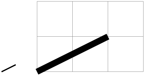
                    \begin{tikzpicture}

                      \draw[help lines] (0,0) grid
                    (3,2);

                      \pgfsetlinewidth{1pt}

                      \begin{pgflowlevelscope}{\pgftransformscale{5}}

                        \draw (0,0) --
                    (0.4,.2);

                      \end{pgflowlevelscope}

                      \begin{pgflowlevelscope}{\pgftransformxshift{-1cm}}

                        \draw (0,0) --
                    (0.4,.2);

                      \end{pgflowlevelscope}

                    \end{tikzpicture}
-
\pgflowlevelscope{⟨transformation code⟩}
-
⟨environment contents⟩
-
\endpgflowlevelscope
Plain TeX version of the environment.
-
\startpgflowlevelscope{⟨transformation code⟩}
-
⟨environment contents⟩
-
\stoppgflowlevelscope
ConTeXt version of the environment.
108.3.2 Establishing View Boxes
A view box is like a “window” through which you see a graphic. To establish a view box, you specify a rectangle – which is the window – and another rectangle surrounding the to-be-viewed graphic. The graphic will then be rescaled and shifted in such a way that the to-be-viewed rectangle matches the view box’s rectangle as well as possible. Note that establishing a view box does, indeed, cause a canvas transformation to be installed.
View boxes are only seldom needed in normal graphics. Their main application is with animations since you can animate the to-be-viewed rectangle. This makes it easy to create animations in which you zoom in, zoom out, and pan a graphic.
-
\begin{pgfviewboxscope}{⟨\(ll_1\)⟩}{⟨\(ur_1\)⟩}{⟨\(ll_2\)⟩}{⟨\(ur_2\)⟩}{⟨meet or slice⟩} 
-
⟨environment contents⟩
-
\end{pgfviewboxscope}
Inside the viewbox scope, the source rectangle (with the two pgf points \(ll_1\) and \(ur_1\) as corners) will be translated and scaled so that it becomes centered on the target rectangle (with the corners \(ll_2\) and \(ur_2\)) and will, for meet as last parameter, be as large as possible so that it fits inside the target and, for slice, be as small as possible so that it encompasses the target.

                    \tikz {

                      \draw [red, very thick] (0,0) rectangle
                    (20mm,20mm);

                      \begin{pgfviewboxscope}

                        {\pgfpoint{5mm}{5mm}}{\pgfpoint{25mm}{15mm}} % Source

                        {\pgfpoint{0mm}{0mm}}{\pgfpoint{20mm}{20mm}} % Target

                        {meet}

                        \draw [blue, very thick] (5mm,5mm) rectangle
                    (25mm,15mm);

                        \draw [thick] (1,1) circle
                    [radius=8mm] node
                    {Hi};

                      \end{pgfviewboxscope} }
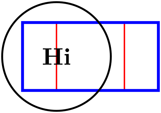
                    \tikz {

                      \draw [red, very thick] (0,0) rectangle
                    (20mm,20mm);

                      \begin{pgfviewboxscope}

                        {\pgfpoint{5mm}{5mm}}{\pgfpoint{25mm}{15mm}} % Source

                        {\pgfpoint{0mm}{0mm}}{\pgfpoint{20mm}{20mm}} % Target

                        {slice}

                        \draw [blue, very thick] (5mm,5mm) rectangle
                    (25mm,15mm);

                        \draw [thick] (1,1) circle
                    [radius=8mm] node
                    {Hi};

                      \end{pgfviewboxscope} }
-
\pgfviewboxscope{⟨\(ll_1\)⟩}{⟨\(ur_1\)⟩}{⟨\(ll_2\)⟩}{⟨\(ur_2\)⟩}{⟨meet or slice⟩}
-
⟨environment contents⟩
-
\endpgfviewboxscope
Plain TeX version of the environment.
-
\startpgfviewboxscope{⟨\(ll_1\)⟩}{⟨\(ur_1\)⟩}{⟨\(ll_2\)⟩}{⟨\(ur_2\)⟩}{⟨meet or slice⟩}
-
⟨environment contents⟩
-
\stoppgfviewboxscope
ConTeXt version of the environment.
108.4 Nonlinear Transformations
In order to use nonlinear transformations, you first have to load the following pgf module:
-
\usepgfmodule{nonlineartransformations} % LaTeX and plain TeX and pure pgf 
-
\usepgfmodule[nonlineartransformations] % ConTeXt and pure pgf
Loads the necessary functionality for nonlinear transformations.
108.4.1 Introduction
The difference between the coordinate transformations introduced in Section 108.2 above to nonlinear transformations is, of course, that the transformations can be nonlinear. An example of a nonlinear transformation is the transformation underlying polar coordinates: A polar coordinate \((r,d)\) gets transformed to the canvas position \((d\cos r,d\sin r)\), which is clearly not a linear transformation.
Nonlinear transformations work somewhat like the normal linear coordinate transformations in the sense that they apply to coordinate and thereby to the construction of paths, but not to things like text or line width or shadings. (Indeed, it is not possible to apply nonlinear transformations to, say, text.)
This means that there is a fundamental difference between, on the one hand, calling a function like \pgfpointpolar or specifying a coordinate as (45:2) in TikZ and, on the other hand, installing the nonlinear transformation “polar coordinates” using the command \pgftransformnonlinear: In a coordinate like (45:2) the user explicitly says “please evaluate this one coordinate in polar coordinate and then continue in the normal coordinate system with the result”. Otherwise nothing changes and a line between two points specified in this way is still a straight line.
Things are quite different when we install a polar transformation using \pgftransformnonlinear. Now, even a seemingly low-level Cartesian coordinate \pgfqpoint{1pt}{1pt} will get transformed. Even more drastically, what is specified as a straight line like
can become curved since everything gets transformed.
108.4.2 Installing Nonlinear Transformation
-
\pgftransformnonlinear{⟨transformation code⟩} 
This command adds the ⟨transformation code⟩ to the list of non-linear transformations currently in force. Thus, similar to linear coordinate transformations, each additional call to this function adds another transformation to the current TeX scope and the effect ends at the end of the current scope. In practice, however, you typically will not have more than one active nonlinear transformation.
The job of the ⟨transformation code⟩ is to map a point \(p\) given in the registers \pgf@x and \pgf@y to a new coordinate \(f(p)\), which should be returned in \pgf@x and \pgf@y as well. As an example, suppose we wish to install polar coordinates as the nonlinear transformation. For this, we need a bit of code:
                    \def\polartransformation{%

                      % \pgf@x will contain the radius

                      % \pgf@y will contain the distance

                      \pgfmathsincos@{\pgf@sys@tonumber\pgf@x}%

                      % pgfmathresultx is now the cosine of radius and

                      % pgfmathresulty is the sine of radius

                      \pgf@x=\pgfmathresultx\pgf@y%

                      \pgf@y=\pgfmathresulty\pgf@y%

                    }
(In case you wonder why you cannot just call \pgfpointpolar at this point: You can, but this function internally uses \pgf@x and \pgf@y in complicated ways, so you would first have to safe them so some other registers. Also, the above is faster.)
If we were to call this function again, we would get something funny like “polar-polar coordinates”, so let’s not do this. Let us instead have a look at the effect this call has: Once a nonlinear transformation is installed, all subsequent path constructions are affected by this transformation. In particular, a normal grid now becomes the typical “polar grid”.
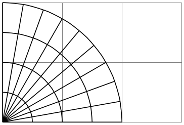
                    \usepgfmodule {nonlineartransformations}

                    \begin{tikzpicture}

                      \draw [help lines] (0,0) grid
                    (3,2);

                      % Start nonlinear transformation

                      \pgftransformnonlinear{\polartransformation}% see above


                      % Draw something with this transformation in force

                      \draw (0pt,0mm) grid
                    [xstep=10pt, ystep=5mm] (90pt, 20mm);

                    \end{tikzpicture}
108.4.3 Applying Nonlinear Transformations to Points
-
\pgfpointtransformednonlinear{⟨point⟩} 
Works like \pgfpointtransformed, but also applies the current nonlinear transformation; that is, it first applies the current linear transformation and then the current nonlinear transformations. Note that, just like \pgfpointtransformed, you normally do not call this function directly since it is called internally by the path drawing commands.
108.4.4 Applying Nonlinear Transformations to Paths
When a nonlinear transformation is installed, the normal path construction commands like \pgfpathmoveto get adjusted so that the “honour” the nonlinear transformations currently in force. For \pgfpathmoveto this is pretty simple: Instead of just applying the linear transformation matrix to the point to which the path should “jump” next, we also apply the nonlinear transformation. However, for a command like \pgfpathlineto, things are much more difficult: A straight line will no longer be a straight line!
In order to make straight lines “bend”, the following changes are in force while a nonlinear transformation is installed:
-
1. Whenever a straight line between two points \(p\) and \(q\) should be added to the path, either through \pgfpathlineto or through \pgfpathclose, we replace this straight line by a “degenerated curve” from \(p\) to \(q\) whose control points are at one third and two third of the distance between \(p\) and \(q\) on the line between \(p\) and \(q\). In this way, while nonlinear transformations are in force, we only need to transform curves.
-
2. Next, suppose we wish to transform a curve from \(p\) to \(q\) with supports \(s\) and \(t\). For this, we simply apply the nonlinear transformation \(f\) to all four points and draw a line with the results. Note that this mapping is actually not quite satisfactory for long lines that are strongly curved:
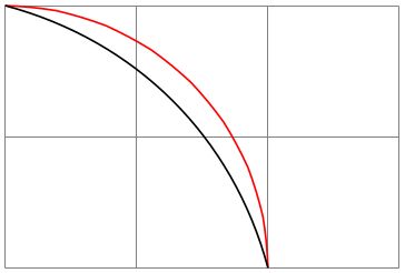
                    \usepgfmodule {nonlineartransformations}

                    \begin{tikzpicture}

                      \draw [help lines] (0,0) grid
                    (3,2);

                      {

                        \pgftransformnonlinear{\polartransformation}

                        % The curve with the controls computed by pgf: a nice quarter arc

                        \draw [red] (0,20mm) --
                    (90pt,20mm);

                      }

                      % Here is the curve with controls just transformed:

                      \draw (0:20mm) .. controls
                    (30pt:20mm) and
                    (60pt:20mm) .. (90pt:20mm);

                    \end{tikzpicture}
As the example shows, the control points now lie on the arc; but in reality they should point along the tangents at the start and the end. This is exactly when pgf does through the computation described above.
-
3. To overcome the effect of the control points being “off”, it is necessary to split up longer curves into smaller parts, which are drawn individually to increase the accuracy. When such splitting occurs, can be configured using the following command:
-
\pgfsettransformnonlinearflatness{⟨dimension⟩} (initially 5pt) 
Whenever in a to-be-drawn curve the \(L^\infty \)-distance (maximum of the distances in \(x\)- and \(y\)-directions) between the start of a curve and its first control point or between the first and second control points or between the second control point and the end is more than ⟨distance⟩, the curve gets split in the middle (more precisely, at time \(t= 0.5\)) and we draw the two parts individually (for them, splitting may occur again, if the curve is still too long).
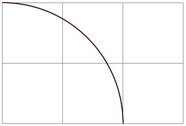
                        \usepgfmodule {nonlineartransformations}

                        \begin{tikzpicture}

                          \draw [help lines] (0,0) grid
                        (3,2);

                          \draw[red] (0:20mm) arc [start angle=0, end angle=90, radius=2cm];

                          {

                            \pgftransformnonlinear{\polartransformation}

                            \pgfsettransformnonlinearflatness{2pt} % very precise

                            \draw (0,20mm) --
                        (90pt,20mm);

                          }

                        \end{tikzpicture}
-
108.4.5 Applying Nonlinear Transformations to Text
Earlier, it was pointed that nonlinear transformations do not apply to text. Nevertheless, when you use \pgftext or \pgfnode, pgf will do a sort of “best effort” to render the text in the nonlinear coordinate system: The point where the text should be shown can obviously be computed easily. When then temporarily reset the nonlinear transformation and, instead, setup a linear transformation that matches the nonlinear transformation at the point where the text should be. Then, the text is shown. This means that if the text is longer, it will not “follow” the nonlinear transformation, but near the origin of the text it will look “correct”. As an example, let us add some text at the grid point of the above example:

                \usepgfmodule {nonlineartransformations}

                \begin{tikzpicture}

                  \draw [help lines] (0,0) grid
                (3,2);

                  \pgftransformnonlinear{\polartransformation}% see above


                  % Draw something with this transformation in force

                  \draw (0pt,0mm) grid
                [xstep=10pt, ystep=5mm] (90pt, 20mm);


                  \foreach \angle in
                {0,30,60,90}

                    \foreach \dist in
                {1,2}

                      {

                        \pgftransformshift{\pgfpoint{\angle pt}{\dist cm}}

                        \pgftext{\angle$^\circ$}

                      }

                \end{tikzpicture}
108.4.6 Approximating Nonlinear Transformations Using Linear Transformations
At any given point, the current nonlinear transformation can be approximated using a linear transformation. The following two functions allow you to install such a local approximation:
-
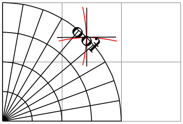
\pgfapproximatenonlineartransformation 
-
1. It clears the nonlinear transformations for the rest of the current TeX scope, so only linear transformations apply.
-
2. However, before removing the nonlinear transformations, the linear transformation matrix is modified so that it mimics the effect the nonlinear transformation had at the origin. That is, after you call this command, drawing something near the origin will look almost the same as if you had not called it.
This command will do two things:
                    \usepgfmodule {nonlineartransformations}

                    \begin{tikzpicture}

                      \draw [help lines] (0,0) grid
                    (3,2);

                      \pgftransformnonlinear{\polartransformation}% see above

                      \draw (0pt,0mm) grid
                    [xstep=10pt, ystep=5mm] (90pt, 20mm);


                      \begin{scope}[shift={(45pt,20mm)}]

                        % Draw something near "origin":

                        \draw [red] (-10pt,-10pt) --
                    (10pt,10pt);

                        \draw [red] (10pt,-10pt) --
                    (-10pt,10pt);


                        % Now draw the same, but in the "approximate" coordinate system:

                        \pgfapproximatenonlineartransformation

                        \draw [] (-10pt,-10pt) --
                    (10pt,10pt);

                        \draw [] (10pt,-10pt) --
                    (-10pt,10pt);

                        \pgftext{foo}

                      \end{scope}

                    \end{tikzpicture}
This command is used by \pgftext and \pgfnode to transform text when a nonlinear transformation is in force.
-
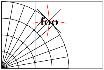
\pgfapproximatenonlineartranslation 
This command works like the normal approximation command, but it will only approximate how the origin gets translated, it will not approximate the rotation, skewing, or scaling that is involved. This is useful for drawing text at the right position, but without “mutilating” the text.
                    \usepgfmodule {nonlineartransformations}

                    \begin{tikzpicture}

                      \draw [help lines] (0,0) grid
                    (3,2);

                      \pgftransformnonlinear{\polartransformation}% see above

                      \draw (0pt,0mm) grid
                    [xstep=10pt, ystep=5mm] (90pt, 20mm);


                      \begin{scope}[shift={(45pt,20mm)}]

                        % Draw something near "origin":

                        \draw [red] (-10pt,-10pt) --
                    (10pt,10pt);

                        \draw [red] (10pt,-10pt) --
                    (-10pt,10pt);


                        % Now draw the same, but in the "approximate" coordinate system:

                        \pgfapproximatenonlineartranslation

                        \draw [] (-10pt,-10pt) --
                    (10pt,10pt);

                        \draw [] (10pt,-10pt) --
                    (-10pt,10pt);

                        \pgftext{foo}

                      \end{scope}

                    \end{tikzpicture}
108.4.7 Nonlinear Transformation Libraries
-
TikZ Library curvilinear 
\usepgflibrary{curvilinear} %
LaTeX
and plain
TeX
and pure pgf
\usepgflibrary[curvilinear] % ConTeXt and pure pgf
\usetikzlibrary{curvilinear} %
LaTeX
and plain
TeX
when using TikZ
\usetikzlibrary[curvilinear] % ConTeXt when using TikZ
This library defines commands for computing nonlinear transformations “along Bézier curves”.
Up to now, our running example for a nonlinear transformation was polar transformation. However, is pgf nonlinear transformations are actually mainly used for transforming arrow tips; and these need to be transformed “along curves”. The curvilinear library defines a number of commands that offer the necessary computations for such transformations.
-
\pgfsetcurvilinearbeziercurve{⟨start⟩}{⟨first support⟩}{⟨second support⟩}{⟨end⟩} 
Prior to using any other command from this library, you first call this function to “install” a Bézier curve to which the commands will refer. This curve will be local to the current TeX scope and you can install only one curve at a time.
The main job of this command is to store the passed points internally and to build a lookup table for distance-to-time conversions, see the next command.
                    \pgfsetcurvilinearbeziercurve

                      {\pgfpointorigin}

                      {\pgfpoint{1cm}{1cm}}

                      {\pgfpoint{2cm}{1cm}}

                      {\pgfpoint{3cm}{0cm}}
-
\pgfcurvilineardistancetotime{⟨distance⟩} 
-
• The conversion will be best near the start of the curve.
-
• The more “degenerate” the curve, the worse the results.
This command does a “distance-to-time-conversion”: It tries to compute a time \(t\), returned in \pgf@x, that corresponds to travelling ⟨distance⟩ along the curve that has last been installed using the command \pgfsetcurvilinearbeziercurve. The distance-to-time-conversion uses the precomputations done by that command. Note that several compromises had to be made between speed and accuracy:
-
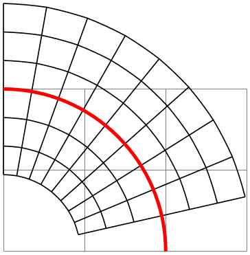
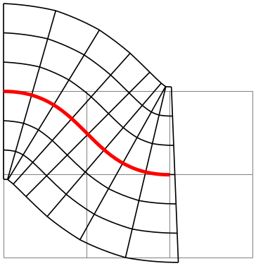
\pgfpointcurvilinearbezierorthogonal{⟨distance⟩}{⟨offset⟩} 
This command computes the following point: Consider the curve last installed using the command \pgfsetcurvilinearbeziercurve. We travel along this curve by ⟨distance⟩, arriving at a point \(p\). Then, we turn by \(90^\circ \) and travel by ⟨offset⟩ units “always from the curve”, arriving at a point \(q\). This point \(q\) will now be returned in \pgf@x and \pgf@y; furthermore, the transformed local coordinate system at point \(q\) will also be returned \pgf@xa and the other registers, see \pgftransformnonlinear for details.
                    \usepgfmodule {nonlineartransformations} \usetikzlibrary {curvilinear}

                    \begin{tikzpicture}

                      \draw [help lines] (0,0) grid
                    (3,2);

                      {

                        \pgfsetcurvilinearbeziercurve

                          {\pgfpoint{0mm}{20mm}}

                          {\pgfpoint{11mm}{20mm}}

                          {\pgfpoint{20mm}{11mm}}

                          {\pgfpoint{20mm}{0mm}}

                        \pgftransformnonlinear{\pgfpointcurvilinearbezierorthogonal\pgf@x\pgf@y}%

                        \draw (0,-30pt) grid
                    [step=10pt] (80pt,30pt);

                      }

                      \draw[red, very thick]

                        (0mm,20mm) .. controls
                    (11mm,20mm) and
                    (20mm,11mm) .. (20mm,0mm);

                    \end{tikzpicture}
                    \usepgfmodule {nonlineartransformations} \usetikzlibrary {curvilinear}

                    \begin{tikzpicture}

                      \draw [help lines] (0,0) grid
                    (3,2);

                      {

                        \pgfsetcurvilinearbeziercurve

                          {\pgfpoint{0mm}{20mm}}

                          {\pgfpoint{10mm}{20mm}}

                          {\pgfpoint{10mm}{10mm}}

                          {\pgfpoint{20mm}{10mm}}

                        \pgftransformnonlinear{\pgfpointcurvilinearbezierorthogonal\pgf@x\pgf@y}%

                        \draw (0,-30pt) grid
                    [step=10pt] (80pt,30pt);

                      }

                      \draw[red, very thick]

                        (0mm,20mm) .. controls
                    (10mm,20mm) and
                    (10mm,10mm) .. (20mm,10mm);

                    \end{tikzpicture}
-
\pgfpointcurvilinearbezierpolar{⟨x⟩}{⟨y⟩} 
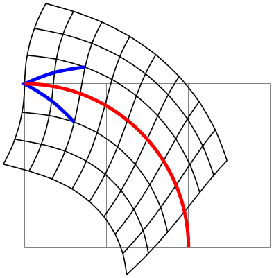
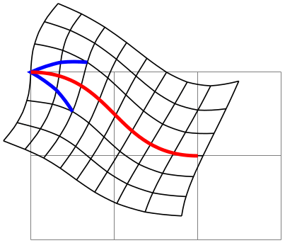
This command is similar to the previous version, but the transformation is different: The idea is that a line form \((0,0)\) to \((x,0)\) gets transformed to the curve from the start of the curve to a point at distance \(x\) along the curve. This is identical to what the “orthogonal” transformation above also does. The difference is that a line from \((0,0)\) to \((0,y)\) gets still transformed to an initial segment of the curve of a length of \(y\), but now rotated by \(90^\circ \). In general, the point \(p = (x,y)\) gets transferred to a point that at distance \(|p| = \sqrt {x^2+y^2}\) along the curve, but rotated by the angle of \(p\) relative to the \(x\)-axis.
All of these computations mainly have the following effect: Two straight lines from the start of the curve as in a Straight Barb arrow tip get transformed to an initial segment of the curve whose length is the length of the two lines, but this segment gets rotated by the angle of the two lines.
                    \usepgfmodule {nonlineartransformations} \usetikzlibrary {curvilinear}

                    \begin{tikzpicture}

                      \draw [help lines] (0,0) grid
                    (3,2);

                      {

                        \pgfsetcurvilinearbeziercurve

                          {\pgfpoint{0mm}{20mm}}

                          {\pgfpoint{11mm}{20mm}}

                          {\pgfpoint{20mm}{11mm}}

                          {\pgfpoint{20mm}{0mm}}

                        \pgftransformnonlinear{\pgfpointcurvilinearbezierpolar\pgf@x\pgf@y}%

                        \draw (0,-30pt) grid
                    [step=10pt] (80pt,30pt);

                        % Add a "barb":

                        \draw [blue, very thick] (20pt,10pt) --
                    (0,0) --
                    (20pt,-10pt);

                      }

                      \draw[red, very thick]

                        (0mm,20mm) .. controls
                    (11mm,20mm) and
                    (20mm,11mm) .. (20mm,0mm);

                    \end{tikzpicture}
                    \usepgfmodule {nonlineartransformations} \usetikzlibrary {curvilinear}

                    \begin{tikzpicture}

                      \draw [help lines] (0,0) grid
                    (3,2);

                      {

                        \pgfsetcurvilinearbeziercurve

                          {\pgfpoint{0mm}{20mm}}

                          {\pgfpoint{10mm}{20mm}}

                          {\pgfpoint{10mm}{10mm}}

                          {\pgfpoint{20mm}{10mm}}

                        \pgftransformnonlinear{\pgfpointcurvilinearbezierpolar\pgf@x\pgf@y}%

                        \draw (0,-30pt) grid
                    [step=10pt] (80pt,30pt);

                        % Add a "barb":

                        \draw [blue, very thick] (20pt,10pt) --
                    (0,0) --
                    (20pt,-10pt);

                      }

                      \draw[red, very thick]

                        (0mm,20mm) .. controls
                    (10mm,20mm) and
                    (10mm,10mm) .. (20mm,10mm);

                    \end{tikzpicture}