Manual for Package pgfplots
2D/3D Plots in LATeX, Version 1.18.1
http://sourceforge.net/projects/pgfplots

\pgfplotstablenew[options]{row count}{\table} ¶

\pgfplotstablenew*[options]{row count}{\table}

Creates a new table from scratch.

The new table will contain all columns listed in the columns key. For \pgfplotstablenew, the columns key needs to be provided in [options]. For \pgfplotstablenew*, the current value of columns is used, no matter where and when it has been set.

Furthermore, there must be create on use statements (see the next subsection) for every column which shall be generated.¹⁰⁶ Columns are generated independently, in the order of appearance in columns. As soon as a column is complete, it can be accessed using any of the basic level access mechanisms. Thus, you can build columns which depend on each other.

The table will contain exactly row count rows. If row count is an \pgfplotstablegetrowsof statement, that statement will be executed and the resulting number of rows be used. Otherwise, row count will be evaluated as number.



copy % this key setting could be provided in the document's preamble: \pgfplotstableset{ % define how the 'new' column shall be filled: create on use/new/.style={create col/set list={4,5,6,7,...,10}}} % create a new table with 11 rows and column 'new': \pgfplotstablenew[columns={new}]{11}\loadedtable % show it: \pgfplotstabletypeset[empty cells with={---}]\loadedtable



copy % create a new table with 11 rows and column 'new': \pgfplotstablenew[ % define how the 'new' column shall be filled: create on use/new/.style={create col/expr={factorial(15+\pgfplotstablerow)}}, columns={new}] {11} \loadedtable % show it: \pgfplotstabletypeset\loadedtable

\pgfplotstablevertcat{\table1}{\table2 or filename} ¶

Appends the contents of \table2 to \table1 (“vertical concatenation”). To be more precise, only columns which exist already in \table1 will be appended and every column which exists in \table1 must exist in \table2 (or there must be alias or create on use specifications to generate them).

If the second argument is a file name, that file will be loaded from disk.

If \table1 does not exist, \table2 will be copied to \table1.

copy \pgfplotstablevertcat{\output}{datafile1} % loads `datafile1' -> `\output' \pgfplotstablevertcat{\output}{datafile2} % appends rows of datafile2 \pgfplotstablevertcat{\output}{datafile3} % appends rows of datafile3

Remark:

The output table \table1 will be defined in the current TeX scope and it will be erased afterwards. The current TeX scope is delimited by an extra set of curly braces. However, every LaTeX environment and, unfortunately, the TikZ \foreach statement as well, introduce TeX scopes.

pgfplots has some some loop statements which do not introduce extra scopes. For example,

These looping macros are explained in the manual of pgfplots, reference section “Miscellaneous Commands”

\pgfplotstableclear{\table} ¶

Clears a table. Note that it is much more reliable to introduce extra curly braces ‘{ ... }’ around table operations – these braces define the scope of a variable (including tables).

\pgfplotstablecreatecol[options]{new col name}{\table} ¶

Creates a new column named new col name and appends it to an already existing table \table.

End users probably don’t need to use \pgfplotstablecreatecol directly at all – there is the high-level framework create on use which invokes it internally and can be used with simple key–value assignments (see below). However, this documentation explains how to use values of existing columns to fill new cells.

This command offers a flexible framework to generate new columns. It has been designed to create new columns using the already existing values – for example using logical or numerical methods to combine existing values. It provides fast access to a row’s value, the previous row’s value and the next row’s value.

The following documentation is for everyone who wants to write specialized columns. It is not particularly difficult; it is just technical and it requires some knowledge of pgfkeys. If you don’t like it, you can resort to predefined column generation styles – and enable those styles in options.

The column entries will be created using the command key create col/assign. It will be invoked for every row of the table. It is supposed to assign contents to create col/next content. During the evaluation, the macro \thisrow{col name} expands to the current row’s value of the column identified by col name. Furthermore, \nextrow{col name} expands to the next row’s value of the designated column and \prevrow{col name} expands to the value of the previous row.

So, the idea is to simply redefine the command key create col/assign in such a way that it fills new cells as desired.

Two special assign routines are available for the first and last row: The contents for the last row is computed with create col/assign last. Its semantics is the same. The contents for the first row is computed with create col/assign first to simplify special cases here. These first and last commands are optional, their default is to invoke the normal assign routine.

The evaluation of the assign keys is done in local TeX groups (i.e. any local definitions will be cleared afterwards).

The following macros are useful during cell assignments:

• 1. \prevrow{col name} / \getprevrow{col name}{\macro}

  These two routines return the value stored in the previous row of the designated column col name. The get routine stores it into \macro.

  The argument col name has to denote either an existing column name or one for which an alias/col name exists.

• 2. \thisrow{col name} / \getthisrow{col name}{\macro}

  These two routines return the current row’s value stored in the designated column. The get routine stores it into \macro.

  The argument col name has to denote either an existing column name or one for which an alias/col name exists.

• 3. \nextrow{col name} / \getnextrow{col name}{\macro}

  These two routines return the next row’s value.

  The argument col name has to denote either an existing column name or one for which an alias/col name exists.

• 4. \pgfplotstablerow and \pgfplotstablerows which contain the current row’s index and the total number of rows, respectively. See page (page for section 6.1.2) for details.

• 5. \pgfmathaccuma and \pgfmathaccumb can be used to transport intermediate results. Both maintain their value from one column assignment to the next. All other local variables will be deleted after leaving the assignment routines. The initial value is the empty string for both of them unless they are already initialized by column creation styles.

• 6. \pgfplotstablename a macro containing the name of the currently processed table (i.e. it contains the second argument of \pgfplotstablecreatecol).

• 7. commands which are valid throughout every part of this package, for example \pgfplotstablerow to get the current row index or \pgfplotstablerows to get the total number of rows.

The col name is expected to be a physical column name, no alias or column index is allowed (unless column indices and column names are the same).

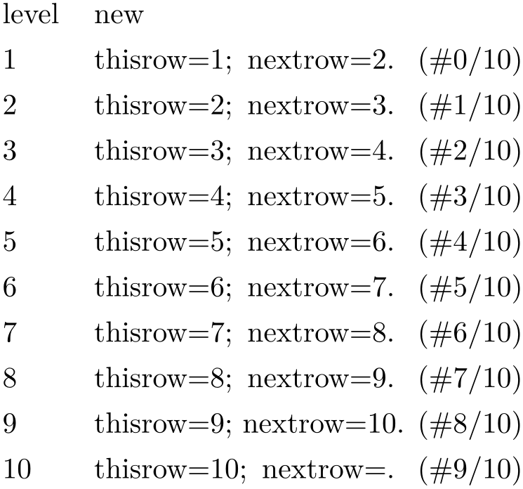
The following example takes our well-known input table and creates a copy of the level column. Furthermore, it produces a lot of output to show the available macros. Finally, it uses \pgfkeyslet to assign the contents of the resulting \entry to next content.



copy \pgfplotstableread{pgfplotstable.example1.dat}\loadedtable \pgfplotstablecreatecol[ create col/assign/.code={% \getthisrow{level}\entry \getnextrow{level}\nextentry \edef\entry{thisrow=\entry; nextrow=\nextentry. (\#\pgfplotstablerow/\pgfplotstablerows)}% \pgfkeyslet{/pgfplots/table/create col/next content}\entry }] {new}\loadedtable \pgfplotstabletypeset[ column type=l, columns={level,new}, columns/new/.style={string type} ]\loadedtable

There is one more specialty: you can use columns={column list} to reduce the runtime complexity of this command. This works only if the columns key is provided directly into options. In this case \thisrow and its variants are only defined for those columns listed in the columns value.

Limitations.

Currently, you can only access three values of one column at a time: the current row, the previous row and the next row. Access to arbitrary indices is not (yet) supported.

Remark:

If you’d like to create a table from scratch using this command (or the related create on use simplification), take a look at \pgfplotstablenew.

The default implementation of assign is to produce empty strings. The default implementation of assign last is to invoke assign, so in case you never really use the next row’s value, you won’t need to touch assign last. The same holds for assign first.

/pgfplots/table/create on use/col name/.style={create options} ¶

Allows “lazy creation” of the column col name. Whenever the column col name is queried by name, for example in an \pgfplotstabletypeset command, and such a column does not exist already, it is created on the fly.



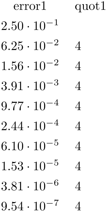
copy % requires \usepackage{array} \pgfplotstableset{% could be used in preamble create on use/quot1/.style= {create col/quotient={error1}}} \pgfplotstabletypeset[ columns={error1,quot1}, columns/error1/.style={sci,sci zerofill}, columns/quot1/.style={dec sep align}] {pgfplotstable.example1.dat}

The example above queries quot1 which does not yet exist in the input file. Therefore, it is checked whether a create on use style for quot1 exists. This is the case, so it is used to create the missing column. The create col/quotient key is discussed below; it computes quotients of successive rows in column error1.

A create on use specification is translated into

\pgfplotstablecreatecol[create options]{col name}{the table},

or, equivalently, into

\pgfplotstablecreatecol[create on use/col name]{col name}{the table}.

This feature allows some laziness, because you can omit the lengthy table modifications. However, laziness may cost something: in the example above, the generated column will be lost after returning from \pgfplotstabletypeset.

The create on use has higher priority than alias.

In case col name contains characters which are required for key settings, you need to use braces around it: “create on use/{name=wi/th,special}/.style={...}”.

More examples for create on use are shown below while discussing the available column creation styles.

Note that create on use is also available within pgfplots, in \addplot table when used together with the read completely key.

/pgfplots/table/create col/set={value} ¶

A style for use in column creation context which creates a new column and writes value into each new cell. The value is written as string (verbatim).



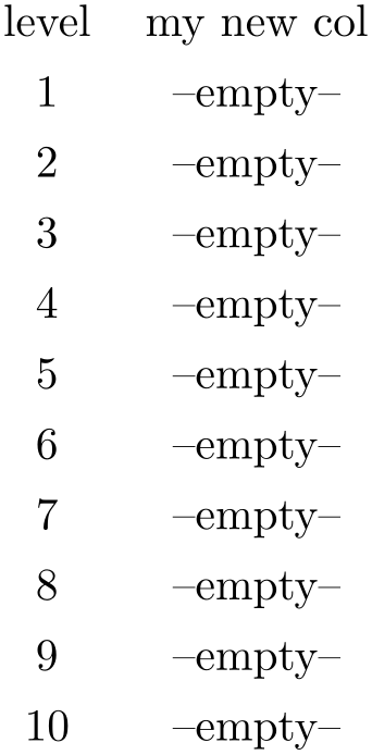
copy \pgfplotstableset{ create on use/my new col/.style={create col/set={--empty--}}, columns/my new col/.style={string type} } \pgfplotstabletypeset[ columns={level,my new col}, ]{pgfplotstable.example1.dat}

/pgfplots/table/create col/set list={comma-separated-list} ¶

A style for use in column creation context which creates a new column consisting of the entries in comma-separated-list. The value is written as string (verbatim).

The comma-separated-list is processed via TikZ’s \foreach command, that means you can use ... expressions to provide number (or character) ranges.



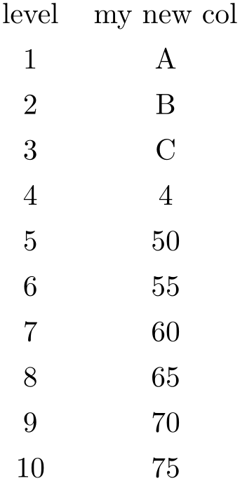
copy \pgfplotstableset{ create on use/my new col/.style={ create col/set list={A,B,C,4,50,55,...,100}}, columns/my new col/.style={string type} } \pgfplotstabletypeset[ columns={level,my new col}, ]{pgfplotstable.example1.dat}

The new column will be padded or truncated to the required number of rows. If the list does not contain enough elements, empty cells will be produced.

/pgfplots/table/create col/copy={column name} ¶

A style for use in column creation context which simply copies the existing column column name.



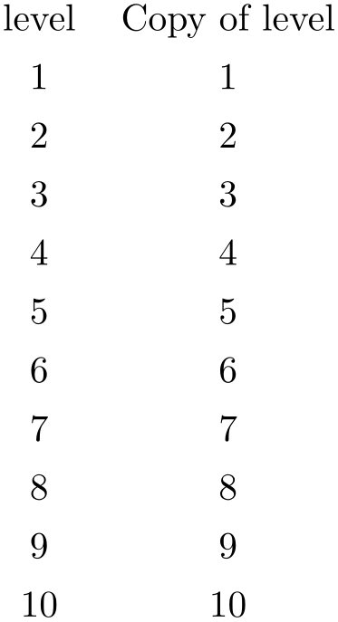
copy \pgfplotstableset{ create on use/new/.style={create col/copy={level}} } \pgfplotstabletypeset[ columns={level,new}, columns/new/.style={column name=Copy of level} ]{pgfplotstable.example1.dat}

/pgfplots/table/create col/copy column from table={file name or \macro}{column name} ¶

A style for use in column creation context which creates a new column consisting of the entries in column name of the provided table. The argument may be either a file name or an already loaded table (i.e. a \macro as returned by \pgfplotstableread).

You can use this style, possibly combined with \pgfplotstablenew, to merge one common sort of column from different tables into one large table.

The cell values are written as string (verbatim).

The new column will be padded or truncated to the required number of rows. If the list does not contain enough elements, empty cells will be produced.

/pgf/fpu=true|false (initially true)

Before we start to describe the column generation methods, one word about the math library. The core is always the pgf math engine written by Mark Wibrow and Till Tantau. However, this engine has been written to produce graphics and is not suitable for scientific computing.

I added a high-precision floating point library to pgf which will be part of releases newer than pgf \(2.00\). It offers the full range of IEEE double precision computing in TeX. This FPU is also part of PgfplotsTable, and it is activated by default for create col/expr and all other predefined mathematical methods.

The FPU won’t be active for newly defined numerical styles (although it is active for the predefined mathematical expression parsing styles like create col/expr). If you want to add own routines or styles, you will need to use

copy \pgfkeys{/pgf/fpu=true}

in order to activate the extended precision. The standard math parser is limited to fixed point numbers in the range of \(\pm 16384.00000\).

/pgfplots/table/create col/expr={math expression} ¶

A style for use in \pgfplotstablecreatecol which uses math expression to assign contents for the new column.



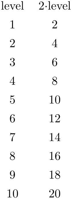
copy \pgfplotstableset{ create on use/new/.style={ create col/expr={\thisrow{level}*2}} } \pgfplotstabletypeset[ columns={level,new}, columns/new/.style={column name=$2\cdot $level} ]{pgfplotstable.example1.dat}

The macros \thisrow{col name} and \nextrow{col name} can be used to use values of the existing table.

Please see \pgfplotstablecreatecol for more information.

Accumulated columns:

The expr style initializes \pgfmathaccuma to 0 before its first column. Whenever it computes a new column value, it redefines \pgfmathaccuma to be the result. That means you can use \pgfmathaccuma inside of math expression to accumulate columns. See create col/expr accum for more details.

About the precision and number range:

Starting with version 1.2, expr uses a floating point unit. The FPU provides the full data range of scientific computing with a relative precision between \(10^{-4}\) and \(10^{-6}\). The /pgf/fpu key provides some more details.

Accepted operations:

The math parser of pgf, combined with the FPU, provides the following function and operators:

+, -, *, /, abs, round, floor, mod, <, >, max, min, sin, cos, tan, deg (conversion from radians to degrees), rad (conversion from degrees to radians), atan, asin, acos, cot, sec, cosec, exp, ln, sqrt, the constanst pi and e, ^ (power operation), factorial¹⁰⁷, rand (random between \(-1\) and \(1\) following a uniform distribution), rnd (random between \(0\) and \(1\) following a uniform distribution), number format conversions hex, Hex, oct, bin and some more. The math parser has been written by Mark Wibrow and Till Tantau, the FPU routines have been developed as part of pgfplots. The documentation for both parts can be found in the PGF/TikZ manual. Attention: Trigonometric functions work with degrees, not with radians, unless trig format is reconfigured!

/pgfplots/table/create col/expr accum={math expression}{accum initial} ¶

A variant of create col/expr which also allows to define the initial value of \pgfmathaccuma. The case accum initial=0 is equivalent to expr={math expression}.



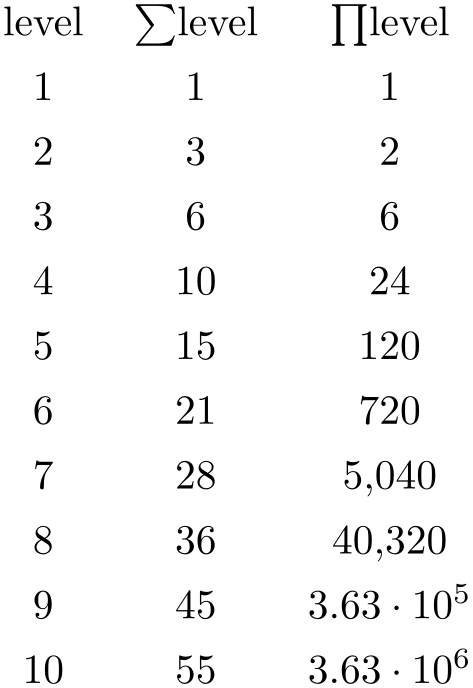
copy \pgfplotstableset{ create on use/new/.style={ create col/expr={\pgfmathaccuma + \thisrow{level}}}, create on use/new2/.style={ create col/expr accum={\pgfmathaccuma * \thisrow{level}}{1}% <- start with `1' } } \pgfplotstabletypeset[ columns={level,new,new2}, columns/new/.style={column name=$\sum$level}, columns/new2/.style={column name=$\prod$level} ]{pgfplotstable.example1.dat}

The example creates two columns: the new column is just the sum of each value in the level column (it employs the default \pgfmathaccuma=0). The new2 column initializes \pgfmathaccuma=100 and then successively subtracts the value of level.

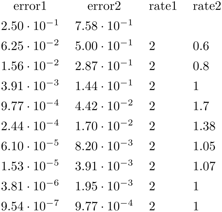
/pgfplots/table/create col/quotient={column name} ¶

A style for use in \pgfplotstablecreatecol which computes the quotient \(c_i := m_{i-1} / m_i\) for every entry \(i = 1,\dotsc , (n-1)\) in the column identified with column name. The first value \(c_0\) is kept empty.



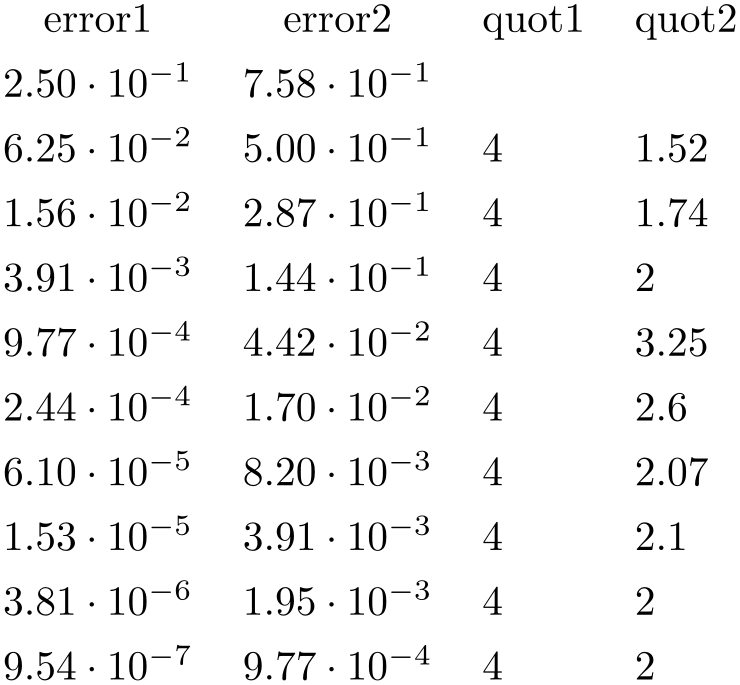
copy % requires \usepackage{array} \pgfplotstableset{% configuration, for example, in preamble: create on use/quot1/.style={create col/quotient=error1}, create on use/quot2/.style={create col/quotient=error2}, columns={error1,error2,quot1,quot2}, % % display styles: columns/error1/.style={sci,sci zerofill}, columns/error2/.style={sci,sci zerofill}, columns/quot1/.style={dec sep align}, columns/quot2/.style={dec sep align} } \pgfplotstabletypeset{pgfplotstable.example1.dat}

This style employs methods of the floating point unit, that means it works with a relative precision of about \(10^{-7}\) (\(7\) significant digits in the mantissa).

/pgfplots/table/create col/iquotient={column name} ¶

Like create col/quotient, but the quotient is inverse.

/pgfplots/table/create col/dyadic refinement rate={column name} ¶

A style for use in \pgfplotstablecreatecol which computes the convergence rate \(\alpha \) of the data in column column name. The contents of column name is assumed to be something like \(e_i(h_i) = O(h_i^\alpha )\). Assuming a dyadic refinement relation from one row to the next, \(h_i = h_{i-1}/2\), we have \(h_{i-1}^\alpha / (h_{i-1}/2)^\alpha = 2^\alpha \), so we get \(\alpha \) using

\[ c_i := \log _2\left ( \frac {e_{i-1}}{e_i} \right ). \]

The first value \(c_0\) is kept empty.



copy % requires \usepackage{array} \pgfplotstabletypeset[% here, configuration options apply only to this single statement: create on use/rate1/.style={create col/dyadic refinement rate={error1}}, create on use/rate2/.style={create col/dyadic refinement rate={error2}}, columns={error1,error2,rate1,rate2}, columns/error1/.style={sci,sci zerofill}, columns/error2/.style={sci,sci zerofill}, columns/rate1/.style={dec sep align}, columns/rate2/.style={dec sep align}] {pgfplotstable.example1.dat}

This style employs methods of the floating point unit, that means it works with a relative precision of about \(10^{-6}\) (\(6\) significant digits in the mantissa).

/pgfplots/table/create col/idyadic refinement rate={column name} ¶

As create col/dyadic refinement rate, but the quotient is inverse.

/pgfplots/table/create col/gradient={col x}{col y} ¶

/pgfplots/table/create col/gradient loglog={col x}{col y} ¶

/pgfplots/table/create col/gradient semilogx={col x}{col y} ¶

/pgfplots/table/create col/gradient semilogy={col x}{col y} ¶

A style for \pgfplotstablecreatecol which computes piecewise gradients \((y_{i+1} - y_i) / (x_{i+1} - x_i )\) for each row. The \(y\) values are taken out of column col y and the \(x\) values are taken from col y.

The logarithmic variants apply the natural logarithm, \(\log (\cdot )\), to its argument before starting to compute differences. More precisely, the loglog variant applies the logarithm to both \(x\) and \(y\), the semilogx variant applies the logarithm only to \(x\) and the semilogy variant applies the logarithm only to \(y\).



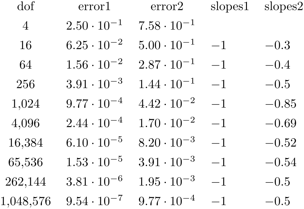
copy % requires \usepackage{array} \pgfplotstableset{% configuration, for example in preamble: create on use/slopes1/.style={create col/gradient loglog={dof}{error1}}, create on use/slopes2/.style={create col/gradient loglog={dof}{error2}}, columns={dof,error1,error2,slopes1,slopes2}, % display styles: columns/dof/.style={int detect}, columns/error1/.style={sci,sci zerofill}, columns/error2/.style={sci,sci zerofill}, columns/slopes1/.style={dec sep align}, columns/slopes2/.style={dec sep align} } \pgfplotstabletypeset{pgfplotstable.example1.dat}



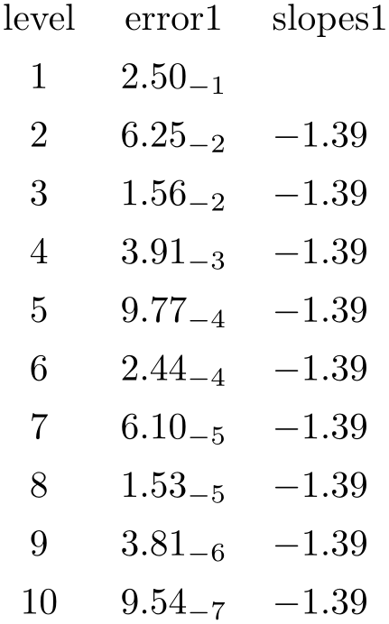
copy % requires \usepackage{array} \pgfplotstableset{% configuration, for example in preamble: create on use/slopes1/.style={create col/gradient semilogy={level}{error1}}, columns={level,error1,slopes1}, % display styles: columns/level/.style={int detect}, columns/error1/.style={sci,sci zerofill,sci subscript}, columns/slopes1/.style={dec sep align} } \pgfplotstabletypeset{pgfplotstable.example1.dat}

This style employs methods of the floating point unit, that means it works with a relative precision of about \(10^{-6}\) (\(6\) significant digits in the mantissa).

/pgfplots/table/create col/linear regression={key-value-config}

Computes a linear (least squares) regression \(y(x) = a \cdot x + b\) using the sample data \((x_i,y_i)\) which has to be specified inside of key-value-config.



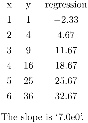
copy % load table from somewhere: \pgfplotstableread{ x y 1 1 2 4 3 9 4 16 5 25 6 36 }\loadedtbl % create the `regression' column: \pgfplotstablecreatecol[linear regression] {regression} {\loadedtbl} % store slope \xdef\slope{\pgfplotstableregressiona} \pgfplotstabletypeset\loadedtbl\\ The slope is `\slope'.

The example above loads a table from inline data, appends a column named ‘regression’ and typesets it. Since no key-value-config has been provided, x=[index]0 and y=[index]1 will be used. The \xdef\slope{...} command stores the ‘\(a\)’ value of the regression line into a newly defined macro ‘\slope’.¹⁰⁸

The complete documentation for this feature has been moved to pgfplots due to its close relation to plotting. Please refer to the pgfplots manual coming with this package.

/pgfplots/table/create col/function graph cut y={cut value}{common options}{one key–value set for each plot} ¶

A specialized style for use in create on use statements which computes cuts of (one or more) discrete plots \(y(x_1), \dotsc , y(x_N)\) with a fixed cut value. The \(x_i\) are written into the table’s cells.

In a cost–accuracy plot, this feature allows to extract the cost for fixed accuracy. The dual feature with cut x allows to compute the accuracy for fixed cost.



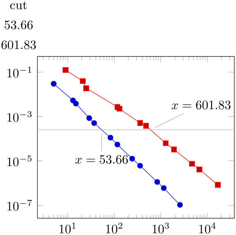
copy % Preamble: \pgfplotsset{width=7cm,compat=1.18} \pgfplotstablenew[ create on use/cut/.style={create col/function graph cut y= {2.5e-4} % search for fixed L2 = 2.5e-4 {x=Basis,y=L2,ymode=log,xmode=log} % double log, each function is L2(Basis) % now, provide each single function f_i(Basis): {{table=plotdata/newexperiment1.dat},{table=plotdata/newexperiment2.dat}} }, columns={cut}] {2} \loadedtable % Show the data: \pgfplotstabletypeset{\loadedtable} \begin{tikzpicture} \begin{loglogaxis} \addplot table[x=Basis,y=L2] {plotdata/newexperiment1.dat}; \addplot table[x=Basis,y=L2] {plotdata/newexperiment2.dat}; \draw[blue!30!white] (1,2.5e-4) -- (1e5,2.5e-4); \node[pin=-90:{$x=53.66$}] at (53.66,2.5e-4) {}; \node[pin=45:{$x=601.83$}] at (601.83,2.5e-4) {}; \end{loglogaxis} \end{tikzpicture}

In the example above, we are searching for \(x_1\) and \(x_2\) such that \(f_1(x_1) = 2.5\cdot 10^{-4}\) and \(f_2(x_2) =2.5\cdot 10^{-4}\). On the left is the automatically computed result. On the right is a problem illustration with proper annotation using pgfplots to visualize the results. The cut value is set to 2.5e-4. The common options contain the problem setup; in our case logarithmic scales and column names. The third argument is a comma-separated-list. Each element \(i\) is a set of keys describing how to get \(f_i(\cdot )\).

During both common options and one key–value set for each plot, the following keys can be used:

• • table={table file or \macro}: either a file name or an already loaded table where to get the data points,

• • x={col name}: the column name of the \(x\)-axis,

• • y={col name}: the column name of the \(y\)-axis.

• • foreach={\foreach loop head}{file name pattern} This somewhat advanced syntax allows to collect tables in a loop automatically:

  

  copy \pgfplotstablenew[ % same as above... create on use/cut/.style={create col/function graph cut y= {2.5e-4}% search for fixed L2 = 2.5e-4 {x=Basis,y=L2,ymode=log,xmode=log, foreach={\i in {1,2}}{plotdata/newexperiment\i.dat}}% {}% just leave this empty. }, columns={cut}] {2} \loadedtable % Show the data: \pgfplotstabletypeset{\loadedtable}

  PgfplotsTable will call \foreach \foreach loop head and it will expand file name pattern for every iteration. For every iteration, a simpler list entry of the form

  table={expanded pattern},x={value of x},y={value of y}

  will be generated.

  It is also possible to provide foreach= inside of one key–value set for each plot. The foreach key takes precedence over table. Details about the accepted syntax of \foreach can be found in the pgf manual.

The keys xmode and ymode can take either log or linear. All mentioned keys have the common key path

/pgfplots/table/create col/function graph cut/.

/pgfplots/table/create col/function graph cut x={cut value}{common options}{one key–value set for each plot} ¶

As above, just with \(x\) and \(y\) exchanged.