Manual for Package pgfplots
2D/3D Plots in LATeX, Version 1.18.2
https://github.com/pgf-tikz/pgfplots
PGFplotsTable
6.1Loading and Displaying data
6.1.1Text Table Input Format
PgfplotsTable works with plain text file tables in which entries (“cells”) are separated by a separation character. The initial separation character is “white space” which means “at least one space or tab” (see option col sep below). Those tables can have a header line which contains column names and most other columns typically contain numerical data.
The following listing shows pgfplotstable.example1.dat and is used often throughout this documentation.
# Convergence results
# fictional source, generated 2008
                level    dof      error1
                           error2   info
                    grad(log(dof),log(error2)) quot(error1)
                1        4        2.50000000e-01
                   7.57858283e-01    48       0
                                0
                2        16       6.25000000e-02
                   5.00000000e-01    25       -3.00000000e-01
                  4
                3        64       1.56250000e-02
                   2.87174589e-01    41       -3.99999999e-01
                  4
                4        256      3.90625000e-03
                   1.43587294e-01    8        -5.00000003e-01
                  4
                5        1024     9.76562500e-04
                   4.41941738e-02    22       -8.49999999e-01
                  4
                6        4096     2.44140625e-04
                   1.69802322e-02    46       -6.90000001e-01
                  4
                7        16384    6.10351562e-05
                   8.20091159e-03    40       -5.24999999e-01
                  4
                8        65536    1.52587891e-05
                   3.90625000e-03    48       -5.35000000e-01
                  3.99999999e+00
                9        262144   3.81469727e-06    1.95312500e-03
                   33       -5.00000000e-01   4.00000001e+00
                10       1048576  9.53674316e-07    9.76562500e-04
                   2        -5.00000000e-01   4.00000001e+00
Lines starting with ‘%’ or ‘#’ are considered to be comment lines and are ignored.
-
\pgfplotstabletypeset[
 optional arguments
 ]{
]{ file name or \macro or inline table
 }
}
Loads (or acquires) a table and typesets it using the current configuration of number formats and table options.
In case the first argument is a file name, the table will be loaded from disk. If it is an already loaded table (see \pgfplotstableread or \pgfplotstablenew), it will be used. Otherwise, if it is inline table data, this data will be parsed just as if it was found in a file (see \pgfplotstableread).
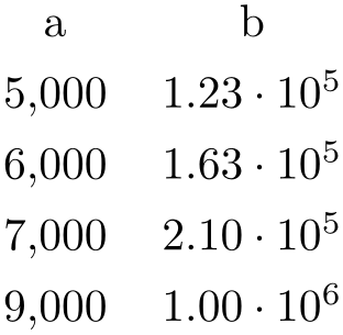

\pgfplotstabletypeset{pgfplotstable.example1.dat}
The configuration can be customized with
 optional arguments
 . Configuration can be done for the complete table or for particular columns (or rows).
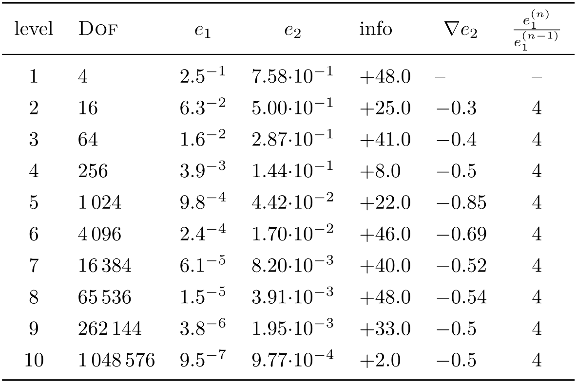
                    \pgfplotstableset{% global config, for example in the
                    preamble
% these columns//.style={} things define a style
% which applies to only.
columns/dof/.style={int detect,column type=r,column name=\textsc{Dof}},
columns/error1/.style={
sci,sci zerofill,sci sep align,precision=1,sci superscript,
column name=$e_1$,
},
columns/error2/.style={
sci,sci zerofill,sci sep align,precision=2,sci 10e,
column name=$e_2$,
},
columns/{grad(log(dof),log(error2))}/.style={
string replace={0}{}, % erase '0'
column name={$\nabla e_2$},
dec sep align,
},
columns/{quot(error1)}/.style={
string replace={0}{}, % erase '0'
column name={$\frac{e_1^{(n)}}{e_1^{(n-1)}}$}
},
empty cells with={--}, % replace empty cells with '--'
every head row/.style={before row=\toprule,after row=\midrule},
every last row/.style={after row=\bottomrule}
}
                    \pgfplotstabletypeset[ % local config,
                    applies only for this table
1000 sep={\,},
columns/info/.style={
fixed,fixed zerofill,precision=1,showpos,
column type=r,
}
]
{pgfplotstable.example1.dat}
All of these options are explained in all detail in the following sections.
You may also use an input format similar to the tabular environment:
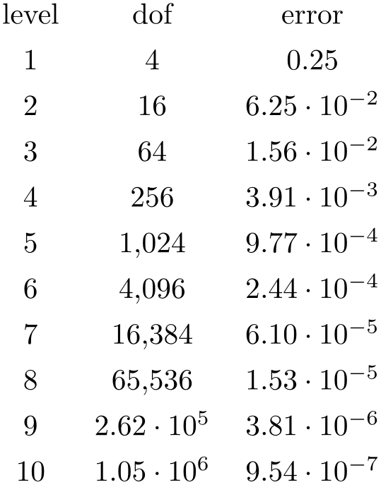
\pgfplotstabletypeset
[col sep=&,row sep=\\,sci zerofill]
{
level & dof & error \\
                        1 &      4 &
                         2.50000000e-01 \\
                        2 &      16 &
                        6.25000000e-02 \\
                        3 &      64 &
                        1.56250000e-02 \\
4 & 256 & 3.90625000e-03 \\
5 & 1024 & 9.76562500e-04 \\
6 & 4096 & 2.44140625e-04 \\
7 & 16384 & 6.10351562e-05 \\
8 & 65536 & 1.52587891e-05 \\
9 & 262144 & 3.81469727e-06 \\
10 & 1048576 &9.53674316e-07 \\
}
Technical note: every opened file will be protocolled into your logfile.
-
\pgfplotstabletypesetfile[
 optional arguments
 ]{
]{ file name
 }
}
Loads the table
 file name
 and typesets it. As of PgfplotsTable 1.2, this command is an alias to
\pgfplotstabletypeset, that means the first argument can be either a file name or an already loaded table.
-
\pgfplotstableread{
 file name
 }{
}{ \macro
 }
}
-
\pgfplotstableread{
 inline table
 }{
}{ \macro
 }
}
Loads a table into the
TeX
macro
 \macro
 . This macro will store the table as internal structure and can be used multiple times.
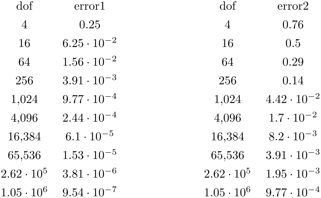
\pgfplotstableread{pgfplotstable.example1.dat}\loadedtable
\pgfplotstabletypeset[columns={dof,error1}]\loadedtable
\hspace{2cm}
\pgfplotstabletypeset[columns={dof,error2}]\loadedtable
The first argument can be a
 file name
 as in the example here. It is also possible to provide the table data directly:
% Alternative: inline table data:
\pgfplotstableread{
                    level   dof     error1  error2  info
                       grad(log(dof),log(error2))      quot(error1)
                    1       4       2.50000000e-01
                     7.57858283e-01  48      0
                                  0
                    2       16      6.25000000e-02  5.00000000e-01
                     25      -3.00000000e-01 4
                    3       64      1.56250000e-02  2.87174589e-01
                     41      -3.99999999e-01 4
                    4       256     3.90625000e-03  1.43587294e-01
                     8       -5.00000003e-01 4
                    5       1024    9.76562500e-04  4.41941738e-02  22
                         -8.49999999e-01 4
                    6       4096    2.44140625e-04  1.69802322e-02  46
                         -6.90000001e-01 4
                    7       16384   6.10351562e-05  8.20091159e-03  40
                         -5.24999999e-01 4
                    8       65536   1.52587891e-05  3.90625000e-03  48
                         -5.35000000e-01 3.99999999e+00
                    9       262144  3.81469727e-06  1.95312500e-03  33
                         -5.00000000e-01 4.00000001e+00
                    10      1048576 9.53674316e-07  9.76562500e-04  2
                          -5.00000000e-01 4.00000001e+00
}\loadedtable
% can be used as above:
\pgfplotstabletypeset[columns={dof,error1}]\loadedtable
\hspace{2cm}
\pgfplotstabletypeset[columns={dof,error2}]\loadedtable
It is checked automatically whether the first argument contains inline data or a file name.
This check whether the first argument is inline data or a file name works as follows: if format=auto, the first argument is considered to be a file name unless it contains the row sep character (see row sep). If format=inline, it is always considered to be inline data. If format=file, it is a file name.
Special cases and more details:
-
• The inline data format is “fragile”. If you experience problems, terminate your tables with ‘\\’ combined with row sep=\\ (the docs for row sep contain alternative ways and more explanation).
-
• There are variants of this command which do not really build up a struct, but which report every line to a “listener”. There is also a struct which avoids protection by TeX scopes. In case you need such things, consider reading the source code comments.
-
• Technical note: every opened file will be protocolled into your logfile.
-
• Note: avoid using ‘\table’ as name, it conflicts with \begin{table} of LaTeX.
-
/pgfplots/table/col sep=space|tab|comma|semicolon|colon|braces|&|ampersand (initially space)
Specifies the column separation character for table reading. The initial choice, space, means “at least one white space”. White spaces are tab stops or spaces (newlines characters always delimit lines).
For example, the file pgfplotstable.example1.csv uses commas as separation characters.
# Convergence results
# fictional source generated 2008
level,dof,error1,error2,info,{grad(log(dof),log(error2))},quot(error1)
1,9,2.50000000e-01,7.57858283e-01,48,0,0
2,25,6.25000000e-02,5.00000000e-01,25,-1.35691545e+00,4
3,81,1.56250000e-02,2.87174589e-01,41,-1.17924958e+00,4
4,289,3.90625000e-03,1.43587294e-01,8,-1.08987331e+00,4
5,1089,9.76562500e-04,4.41941738e-02,22,-1.04500712e+00,4
6,4225,2.44140625e-04,1.69802322e-02,46,-1.02252239e+00,4
7,16641,6.10351562e-05,8.20091159e-03,40,-1.01126607e+00,4
8,66049,1.52587891e-05,3.90625000e-03,48,-1.00563427e+00,3.99999999e+00
9,263169,3.81469727e-06,1.95312500e-03,33,-1.00281745e+00,4.00000001e+00
10,1050625,9.53674316e-07,9.76562500e-04,2,-1.00140880e+00,4.00000001e+00
Thus, we need to specify col sep=comma when we read it.
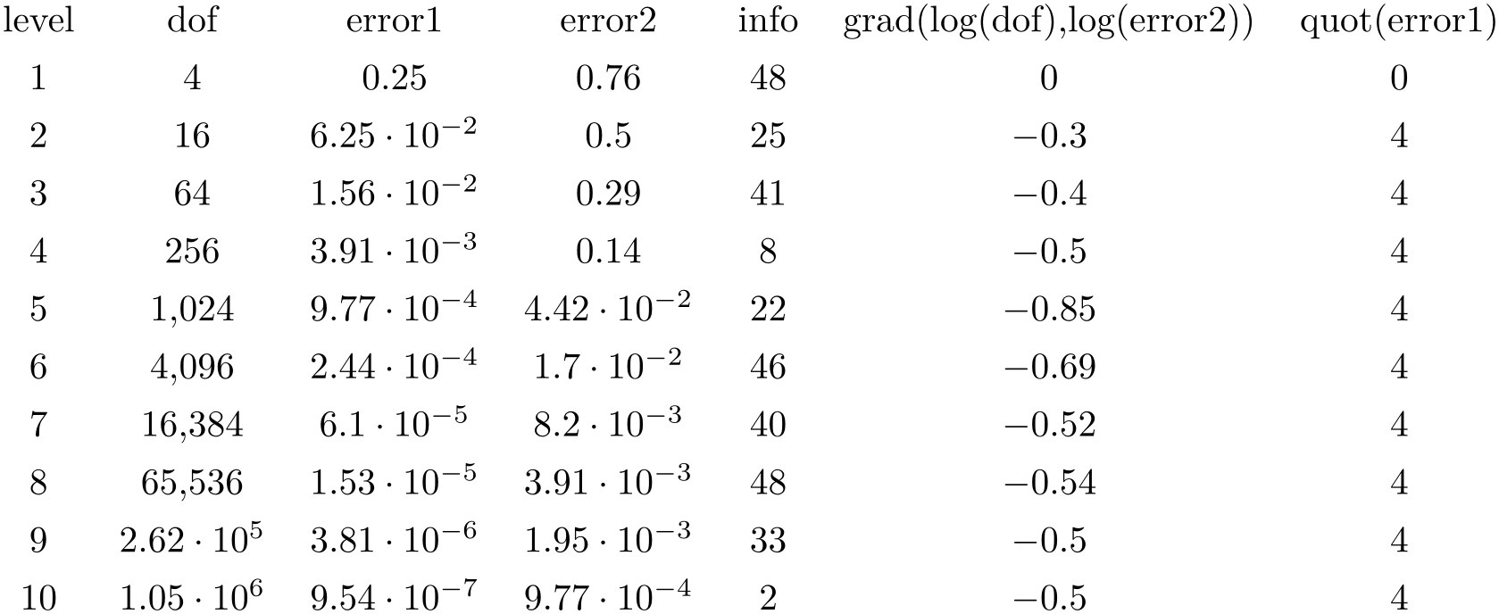
\pgfplotstabletypeset[col sep=comma]{pgfplotstable.example1.csv}
You may call \pgfplotstableset{col sep=comma} once in your preamble if all your tables use commas as column separator.
Please note that if cell entries (for example column names) contain the separation character, you need to enclose the column entry in braces: {grad(log(dof),log(error2)}. If you want to use unmatched braces, you need to write a backslash before the brace. For example the name ‘column{withbrace’ needs to be written as ‘column\{withbrace’.
For col sep\(\neq \)space, spaces will be considered to be part of the argument (there is no trimming). However, (as usual in TeX), multiple successive spaces and tabs are replace by a single white space. Of course, if col sep=tab, tabs are the column separators and will be treated specially.
Furthermore, if you need empty cells in case col sep=space, you have to provide {} to delimit such a cell since col sep=space uses at least one white space (consuming all following ones).
The value col sep=braces is special since it
actually uses two separation characters. Every single cell entry is delimited by an opening and a closing brace,
 entry
entry , for this choice. Furthermore, any white space (spaces and tabs) between cell entries are skipped in case
braces until the next
 entry
entry is found.
A further specialty of col sep=braces is that it has support for multi-line cells: everything within balanced braces is considered to be part of a cell. This includes newlines:100
The col sep=& case (probably together with row sep=\\) allows to read tables as you’d usually type them in LaTeX. This will automatically enable trim cells.
-
/pgfplots/table/header=true|false|has colnames (initially true)
Configures if column names shall be identified automatically during input operations.
The first non-comment line can be a header which contains column names. The header key configures how to detect if that is really the case.
The choice true enables auto detection of column names: If the first non-comment line contains at least one non-numerical entry (for example ‘a name’), each entry in this line is supposed to be a column name. If the first non-comment line contains only numerical data, it is used as data row. In this case, column indices will be assigned as column “names”.
The choice false is identical to this last case, i.e. even if the first line contains strings, they won’t be recognised as column names.
Finally, the choice has colnames is the opposite of false: it assumes that the first non-comment line contains column names. In other words: even if only numbers are contained in the first line, they are considered to be column names.
Note that this key only configures headers in input tables. To configure output headers, you may want to look at every head row.
-
/pgfplots/table/format=auto|inline|file (initially auto) 
Configures the format expected
as first argument for \pgfplotstableread{ input
input }.
}.
The choice inline expects the table data directly as argument where rows are separated by row sep. Inline data is “fragile”, because TeX may consume end-of-line characters (or col sep characters). See row sep for details.
The choice file expects a file name.
The choice auto searches for a row sep in the first argument supplied to \pgfplotstableread. If a row sep has been found, it is inline data, otherwise it is a file name.
-
/pgfplots/table/row sep=newline|\\ (initially newline)
-
1. First possibility: call \pgfplotstableread{
 data
data }\yourmacro outside of any macro declaration.
-
2. Use row sep=\\.
Configures the character to separate rows of the inline table data format (see format=inline).
The choice newline uses the end of line as it appears in the table data (i.e. the input file or any inline table data).
The choice \\ uses ‘\\’ to indicate the end of a row.
Note that newline for inline table data is “fragile”: you can’t provide such data inside of TeX macros (this does not apply to input files). Whenever you experience problems, proceed as follows:
The same applies if you experience problems with inline data and special col sep choices (like col sep=tab).
The reasons for such problems is that TeX scans the macro bodies and replaces newlines by white space. It does other substitutions of this sort as well, and these substitutions can’t be undone (maybe not even found).
-
/pgfplots/table/ignore chars={
 comma-separated-list
 } (initially empty)
Allows to define an “ignore list” for single characters. Any characters found in an input file which occur also
in
 comma-separated-list
 will silently by thrown away. The processing is exactly the same as if you did not write them at all in the first place.
For example, suppose we are given pgfplotstable.example5.dat with
first,second
(1)(0),2 1#2)
(3)(0),4 1#3)
(5)(0),6 1#3)
then, we can ignore several of the characters by writing
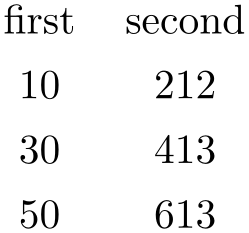
The
 comma-separated-list
 should contain exactly one character in each list element, and the single characters should be separated by commas. Some
special characters like commas, white space, hashes, percents or backslashes need to be escaped by prefixing them with a
backslash.
Besides normal characters, it is also supported to eliminate any binary code from your input files. For example, suppose you have binary characters of code 0x01 (hex notation) in your files. Then, use
\pgfplotstableset{ignore chars={\^^01}}
to eliminate them silently. The ^^ digit
digit
 digit
digit notation is a
TeX
feature to provide characters in hexadecimal encoding where
 digit
digit is one of 0123456789abcdef. I don’t know if the backslash in \^^01 is always necessary, try it
out. There is also a character based syntax, in which \^^M is
 newline
 and \^^I is
 tab
tab . Refer to [4] for more details.
Note that after stripping all these characters, the input table must be valid – it should still contain column separators and balanced columns.
This setting applies to \addplot table and \addplot file for pgfplots as well.
Note that ignore chars is “fragile” when it is applied to format=inline or format=auto. Consider format=file if you experience problems.101
-
/pgfplots/table/white space chars={
 comma-separated-list
 } (initially empty)
Allows to define a list of single characters which are actually treated like white space (in addition to tabs and spaces). It might be useful in order to get more than one column separator character.
The white space chars list is used in exactly the same way as ignore chars, and the same remarks as above apply as well.
-
/pgfplots/table/text special chars={
 comma-separated-list
 } (initially empty)
Allows to define a list of single characters which are actually treated like normal text (like any characters with category code \(12\)).
The text special chars list is used in exactly the same way as ignore chars, and the same remarks as above apply as well.
Note that some (selected) special characters are installed by verb string type.

-
/pgfplots/table/comment chars={
 comma-separated-list
 } (initially empty)
Allows to add one or more additional comment characters. Each of these characters has a similar effect as the # character, i.e. all following characters of that particular input line are skipped.
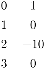
The example above uses ‘!’ as additional comment character (which allows to parse Touchstone files).
-
/pgfplots/table/percent is letter=true|false (initially false) 
Allows to control how to treat percent characters in input files. PgfplotsTable used to keep the TeX special meaning as comment character which means that all characters following percent where ignored.
The value true means that a percent is just a normal letter without special meaning. The value false means that percent is special as it used to be.
-
/pgfplots/table/text indicator={
 char
char } (initially empty)
Allows to define a text indicator character. If this is defined, it can be used to enclose delimiters in a cell’s body:

If the text indicator also occurs within the cell, it has to be doubled:

Cells which do not start with the text indicator are handled normally. Note that text indicator does not support multi-line cells.
-
/pgfplots/table/skip first n={
 integer
 } (initially 0)
Allows to skip the first
 integer
 lines of an input file. The lines will not be processed.
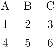
\pgfplotstabletypeset[skip first n=4]{% <- this '%' is important. Otherwise, the
                                                          %
                    newline here would delimit an (empty) row.
XYZ Format,
Version 1.234
Date 2010-09-01
@author Mustermann
A B C
1 2 3
4 5 6
}
-
/pgfplots/table/search path={
 comma-separated-list
 } (initially .)
Allows to provide a search path for input tables. This variable is evaluated whenever pgfplots attempts to read a data file. This includes both \pgfplotstableread and \addplot table; its value resembles a comma-separated list of path names. The requested file will be read from the first matching location in that list.
Use ‘.’ to search using the normal TeX file searching procedure (i.e. typically in the current working directory).
An entry in
 comma-separated-list
 can be relative to the current working directory, i.e. something like
search path={.,../datafiles} is accepted.
-
/pgfplots/table/search path/implicit .=true|false (initially true)
PgfplotsTable allows to add ‘.’ to the value of search path implicitly as this is typically assumed in many applications of search paths.
The initial configuration search path/implicit .=true will ensure that ‘.’ is added in front of the search path if the user value does not contain a ‘.’.
The value search path/implicit .=false will not add ‘.’.
Keep in mind that ‘.’ means “let TeX search for the file on its own”. This will typically find files in the current working directory, but it will also include processing of TEXINPUTS.
100 This treatment of newlines within balanced braces actually applies to every other column separator as well (it is a TeX readline feature). In other words: you can have multi-line cells for every column separator if you enclose them in balanced curly braces. However, col sep=braces has the special treatment that end-of-line counts as white space character; for every other col sep value, this white space is suppressed to remove spurious spaces.
101 See also row sep for more information about dealing with fragile inline table formats.
6.1.2Selecting Columns and their Appearance Styles
-
/pgfplots/table/columns={
 comma-separated-list
 }
}
Selects particular columns of the table. If this option is empty (has not been provided), all available columns will be selected.
Inside of
 comma-separated-list
 , column names as they appear in the table’s header are expected. If there is no header, simply use column indices.
If there are column names, the special syntax [index]
 integer
 can be used to select columns by index. The first column has index \(0\).
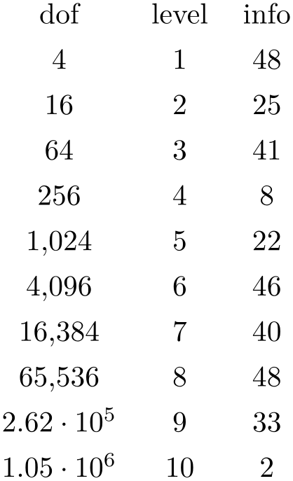
\pgfplotstabletypeset[columns={dof,level,[index]4}]{pgfplotstable.example1.dat}
The special pgfkeys feature \pgfplotstableset{columns/.add={}{,a further col}} allows to append a value, in this case ‘,a further col’ to the actual value. See /.add for details.
-
/pgfplots/table/alias/
 col name
 /.initial={
 real col name
 }
}
Assigns the new name
 col name
 for the column denoted by
 real col name
 . Afterwards, accessing
 col name
 will use the data associated with column
 real col name
 .
.
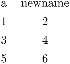
% in preamble:
\pgfplotstableset{
alias/newname/.initial=b,
}
% in document:
\pgfplotstabletypeset[
                        columns={a,newname},%
                    access to `newname' is the same as to `b'
]{
a b
1 2
3 4
5 6
}%
You can use columns/ col name
 /.style to assign styles for the alias, not for the
original column name.
If there exists both an alias and a column of the same name, the column name will be preferred. Furthermore, if there exists a create on use statement with the same name, this one will also be preferred.
In case
 col name
 contains characters which are required for key settings, you need to use braces around it: “alias/{name=wi/th,special}/.initial={othername}”.
This key is used whenever columns are queried, it applies also to the \addplot table statement of pgfplots.
-
/pgfplots/table/columns/
 column name
 /.style={
 key-value-list
 }
}
Sets all options in
 key-value-list
 exclusively for
 column name
 .
.
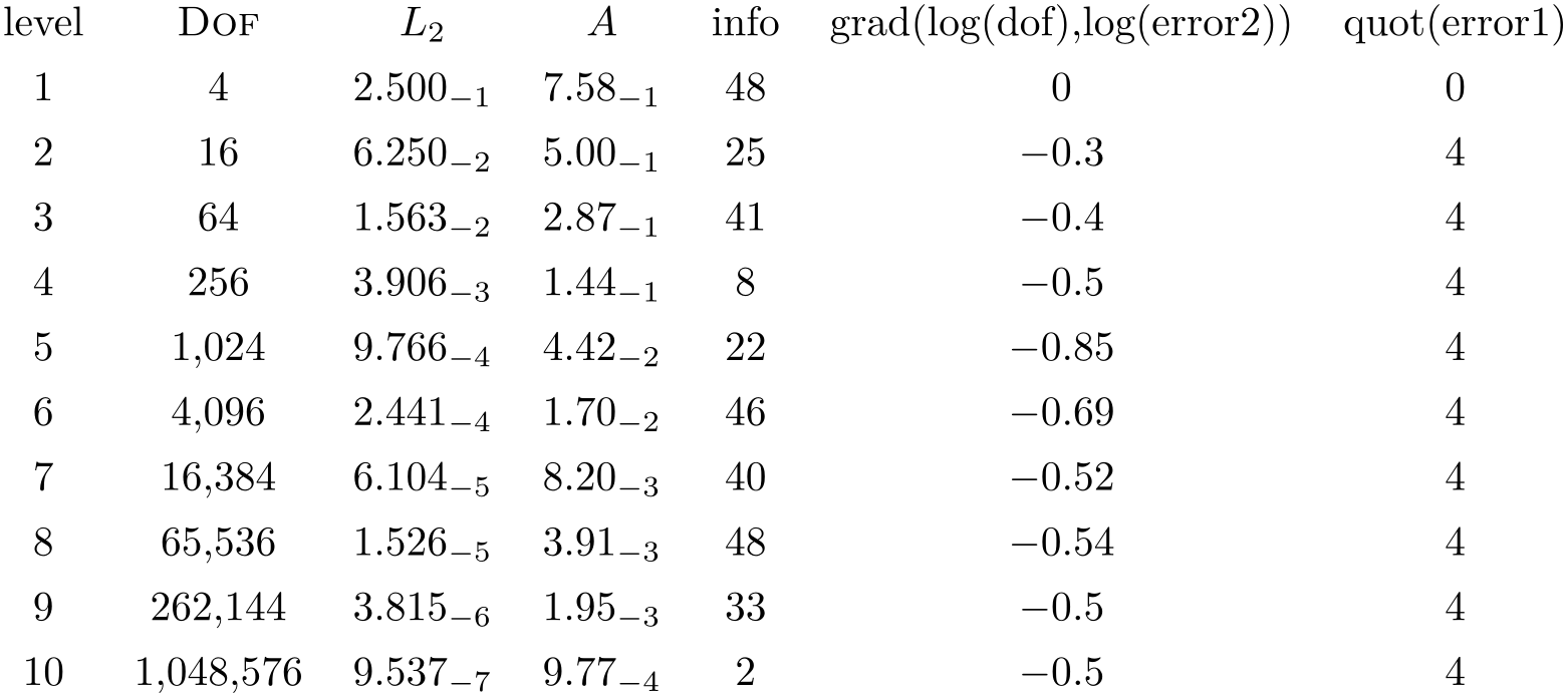
\pgfplotstabletypeset[
columns/error1/.style={
column name=$L_2$,
sci,sci zerofill,sci subscript,
precision=3},
columns/error2/.style={
column name=$A$,
sci,sci zerofill,sci subscript,
precision=2},
columns/dof/.style={
int detect,
column name=\textsc{Dof}
}
]
{pgfplotstable.example1.dat}
If your column name contains commas ‘,’, slashes ‘/’ or equal signs ‘=’, you need to enclose the column name in braces.
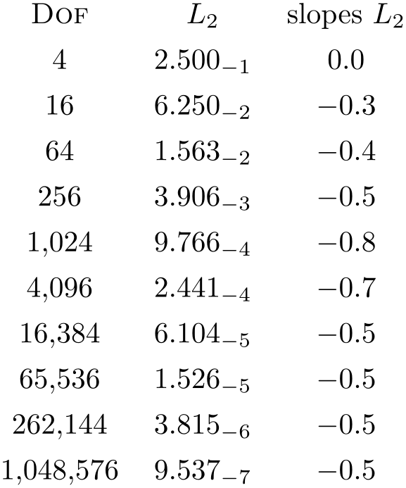
\pgfplotstabletypeset[
columns={dof,error1,{grad(log(dof),log(error2))}},
columns/error1/.style={
column name=$L_2$,
sci,sci zerofill,sci subscript,
precision=3},
columns/dof/.style={
int detect,
column name=\textsc{Dof}},
columns/{grad(log(dof),log(error2))}/.style={
column name=slopes $L_2$,
fixed,fixed zerofill,
precision=1}
]
{pgfplotstable.example1.dat}
If your tables don’t have column names, you can simply use integer indices instead of
 column name
 to refer to columns. If you have column names, you can’t set column styles using indices.
-
/pgfplots/table/display columns/
 index
index /.style={
 key-value-list
 }
}
Applies all options in
 key-value-list
 exclusively to the column which will appear at position
 index
index in the output table.
In contrast to the table/columns/ name
name styles, this option refers to the output table instead of the input table. Since the output table has no unique column name,
you can only access columns by index.
Indexing starts with \(\meta {index}=0\).
Display column styles override input column styles.
-
/pgfplots/table/every col no
 index
index (style, no value)
A style
which is identical with display columns/ index
index : it applies exclusively to the column at position
 index
index in the output table.
See display columns/ index
index for details.
-
/pgfplots/table/column type={
 tabular column type
 } (initially c)
Contains the column type for tabular.
If all column types are empty, the complete argument is skipped (assuming that no tabular environment is generated).
Use
\pgfplotstableset{column type/.add={ before
 }{
}{ after
after }} to modify a value instead of overwriting it. The
/.add key handler works for other options as well.
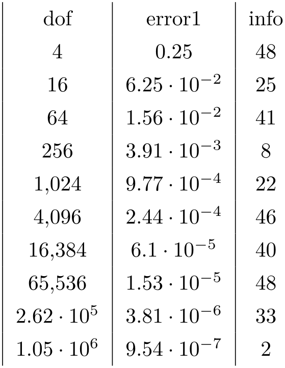
\pgfplotstabletypeset[
columns={dof,error1,info},
column type/.add={|}{}% results in '|c'
]
{pgfplotstable.example1.dat}
-
/pgfplots/table/column name={
 TeX
display column name
 } (initially \pgfkeysnovalue)
Sets the column’s display name in the current context.
It is advisable to provide this option inside of a column-specific style, i.e. using
columns/{ lowlevel colname
 }/.style={column name={
 TeX
display column name
 }} .
}} .
Here, “lowlevel colname” refers to the column name that is present in your input table. This lowlevel column name has a couple of restrictions (it has to be expandable, for example – that means many control sequences are forbidden). The value of column name is only used within \pgfplotstabletypeset in order to generate a display name for the column in question.
Note that you are allowed to provide an empty display name using column name={}. This results in an empty string above the column when used in \pgfplotstabletypeset.
The initial configuration is column name=\pgfkeysnovalue. This constitutes a special “null” value which tells \pgfplotstabletypeset that it should fall back to the column’s name (i.e. the lowlevel name).
Allows to modify the value of column name.
Argument #1 is the current column name, that means after evaluation of column name. After assign column name, a new (possibly modified) value for column name should be set.
That means you can use column name to assign the name as such and assign column name to generate final TeX code (for example to insert \multicolumn{1}{c}{#1}).
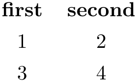
\pgfplotstabletypeset[
assign column name/.style={
/pgfplots/table/column name={\textbf{#1}}
},
]
{
first second
1 2
3 4
}
Note that the PgfplotsTable provides limited postprocessing capabilities for headers, in particular, postproc cell content and its friends merely apply to “normal” cells. If you want to modify the appearance of header cells, you should consider using assign column name.
Default is empty which means no change.
-
/pgfplots/table/multicolumn names={
 tabular column type
 } (style, initially c)
A style which
typesets each column name in the current context using a \multicolumn{1}{ tabular column type
 }{
}{ the column name
 } statement.
Here, the column name
 is set with column name as usual.
-
/pgfplots/table/dec sep align={
 header column type
 } (style, initially c)
A style which aligns numerical columns at the decimal separator.
The first argument determines the alignment of the header column.
Please note that you need \usepackage{array} for this style.
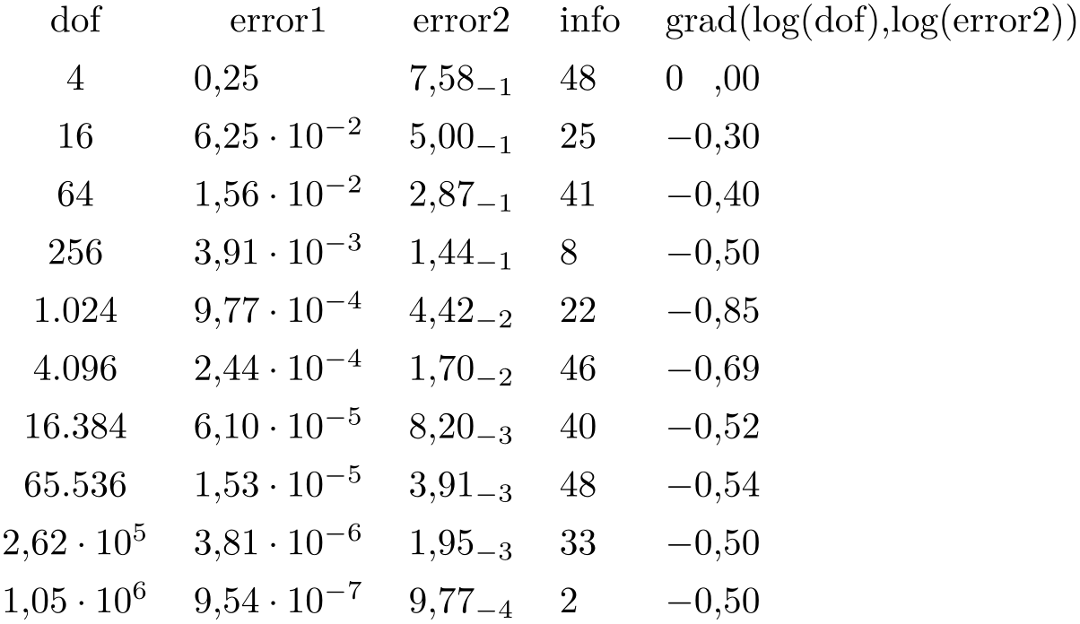
% requires \usepackage{array}
\pgfplotstabletypeset[
columns={dof,error1,error2,info,{grad(log(dof),log(error2))}},
columns/error1/.style={dec sep align},
                        columns/error2/.style={sci,sci
                    subscript,sci zerofill,dec sep align},
columns/info/.style={fixed,dec sep align},
columns/{grad(log(dof),log(error2))}/.style={fixed,dec sep align}
]
{pgfplotstable.example1.dat}
Or with comma as decimal separator:
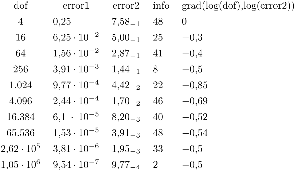
% requires \usepackage{array}
\pgfplotstabletypeset[
use comma,
columns={dof,error1,error2,info,{grad(log(dof),log(error2))}},
columns/error1/.style={dec sep align},
                        columns/error2/.style={sci,sci
                    subscript,sci zerofill,dec sep align},
columns/info/.style={fixed,dec sep align},
columns/{grad(log(dof),log(error2))}/.style={fixed,dec sep align}
]
{pgfplotstable.example1.dat}
It may be advisable to use fixed zerofill and/or sci zerofill to force at least one digit after the decimal separator to improve placement of exponents:
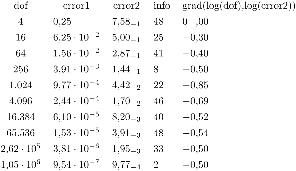
% requires \usepackage{array}
\pgfplotstabletypeset[
use comma,
columns={dof,error1,error2,info,{grad(log(dof),log(error2))}},
columns/error1/.style={dec sep align,sci zerofill},
                        columns/error2/.style={sci,sci
                    subscript,sci zerofill,dec sep align},
columns/info/.style={fixed,dec sep align},
columns/{grad(log(dof),log(error2))}/.style={fixed,dec sep align,fixed zerofill}
]
{pgfplotstable.example1.dat}
The style dec sep align actually introduces two new tabular columns,102 namely r@{}l. It introduces multicolumns for column names accordingly and handles numbers which do not have a decimal separator.
Note that for fixed point numbers, it might be an alternative to use fixed zerofill combined with column type=r to get a similar effect.
Please note that this style overwrites column type, assign cell content and some number formatting settings.
-
/pgfplots/table/sci sep align={
 header column type
 } (style, initially c)
A style which aligns numerical columns at the exponent in scientific representation.
The first argument determines the alignment of the header column.
It works similarly to dec sep align, namely by introducing two artificial columns r@{}l for alignment.
Please note that you need \usepackage{array} for this style.
Please note that this style overwrites column type, assign cell content and some number formatting settings.
-
/pgfplots/table/dcolumn={
 tabular column type
 }{
}{ type for column name
 } (style, initially {D{.}{.}{2}}{c})
A style which can be used together with the dcolumn package of David Carlisle. It also enables alignment at the decimal separator. However, the decimal separator needs to be exactly one character which is incompatible with ‘{,}’ (the default setting for use comma).
-
/pgfplots/table/sort={
 true,false
 } (initially false)
If set to true, \pgfplotstabletypeset will sort the table before applying its operation.
See the description of \pgfplotstablesort for how to configure sort key and sort cmp.

\pgfplotstabletypeset[
sort,sort key=error2,
columns={dof,error1,error2},
                        columns/error1/.style={sci,sci
                    subscript,sci zerofill,dec sep align},
                        columns/error2/.style={sci,sci
                    subscript,sci zerofill,dec sep align},
]
{pgfplotstable.example1.dat}
The sort mechanism is applied before the actual typesetting routine starts, i.e. it has the same effect as if you’d call \pgfplotstablesort manually before typesetting the table (however, the sort key has the advantage of respecting the include outfiles caching mechanism). Any create on use specifications are resolved before calling the sort key.
-
/pgfplots/table/every first column(style, no value) 
A style which is installed for every first column only.
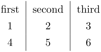
\pgfplotstabletypeset[
every head row/.style={before row=\hline,after row=\hline\hline},
every last row/.style={after row=\hline},
every first column/.style={
column type/.add={|}{}
},
every last column/.style={
column type/.add={}{|}
}]
{pgfplotstable.example1.dat}
-
/pgfplots/table/every last column(style, no value) 
-
/pgfplots/table/every even column(style, no value) 
A style which is installed for every column with even column index (starting with \(0\)).
\pgfplotstableset{
columns={dof,error1,{grad(log(dof),log(error2))},info},
columns/error1/.style={
column name=$L_2$,
sci,sci zerofill,sci subscript,
precision=3},
columns/dof/.style={
int detect,
column name=\textsc{Dof}},
columns/{grad(log(dof),log(error2))}/.style={
column name=slopes $L_2$,
fixed,fixed zerofill,
precision=1}}
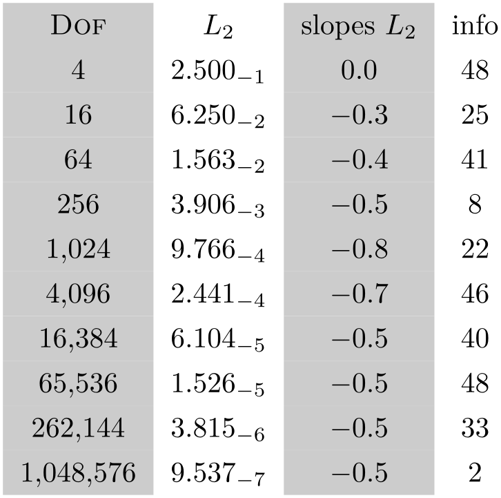
% requires \usepackage{colortbl}
\pgfplotstabletypeset[
every even column/.style={
column type/.add={>{\columncolor[gray]{.8}}}{}
}]
{pgfplotstable.example1.dat}
-
/pgfplots/table/every column(style, no value) 
A style which is applied to every column.
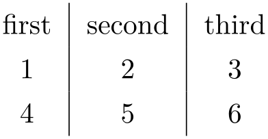
\pgfplotstabletypeset[
every column/.code={
\ifnum\pgfplotstablecol>0
                                \pgfkeysalso{column
                    type/.add={|}{}}%
\fi
},
]
{
first second third
1 2 3
4 5 6
}
-
/pgfplots/table/every odd column(style, no value) 
A style which is installed for every column with odd column index (starting with \(0\)).
-
\pgfplotstablecol 
During the evaluation of row or column options, this command expands to the current column’s index.
-
\pgfplotstablecolname 
During the evaluation of column options, this command expands to the current column’s name. It is valid while \pgfplotstabletypeset processes the column styles (including the preprocessing step explained in Section 6.2.3), prepares the output cell content and checks row predicates.
-
\pgfplotstablerow 
During the evaluation of row or column options, this command expands to the current row’s index.
“Evaluation of column options” applies to any of the styles in Section 6.2, i.e. preprocessing, typesetting, and postprocessing.
The macro \pgfplotstablerow can take any of the values \(0,1,2,\dotsc ,n-1\) where \(n\) is the value of \pgfplotstablerows.
“Evaluation of row options” applies to stuff like every last row.
Note that it will have the special value \(-1\) for the header row.
-
\pgfplotstablecols 
During the evaluation of row or column options, this command expands to the total number of columns in the output table.
-
\pgfplotstablerows 
During evaluation of columns, this command expands to the total number of input rows. You can use it inside of row predicate.
During evaluation of rows, this command expands to the total number of output rows.
-
\pgfplotstablename 
During \pgfplotstabletypeset, this macro contains the table’s macro name as top-level expansion. If you are unfamiliar with “top-level-expansions” and ‘\expandafter’, you will probably never need this macro.
Advances users may benefit from expressions like
\expandafter\pgfplotstabletypeset\pgfplotstablename.
For tables which have been loaded from disk (and have no explicitly assigned macro name), this expands to a temporary macro.
102 Unfortunately, dec sep align is currently not very flexible when it comes to column type modifications. In particular, it is not possible to use colored columns or cells in conjunction with dec sep align. The \rowcolor command works properly; the color hangover introduced by colortbl is adjusted automatically.
6.1.3Configuring Row Appearance: Styles
The following styles allow to configure the final table code after any cell contents have been assigned.
-
/pgfplots/table/before row={
 TeX
code
 }
}
Contains TeX code which will be installed before the first cell in a row.
Keep in mind that PgfplotsTable does no magic – it is simply a code generator which produces tabular environments. Consequently, you can add any TeX code which you would normally write into your tabular environment here.
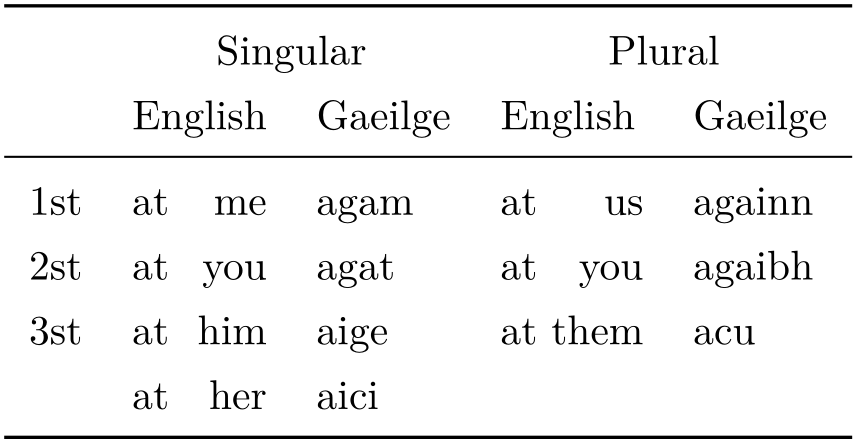
An example could be a multicolumn heading for which PgfplotsTable has no own solution:
% \usepackage{booktabs}
\pgfplotstabletypeset[
column type=l,
every head row/.style={
before row={
\toprule
                                &
                    \multicolumn{2}{c}{Singular} & \multicolumn{2}{c}{Plural}\\
},
after row=\midrule,
},
every last row/.style={
after row=\bottomrule},
columns/person/.style ={column name=},
columns/singGaeilge/.style ={column name=Gaeilge},
columns/pluralGaeilge/.style={column name=Gaeilge},
columns/singEnglish/.style ={column name=English},
columns/pluralEnglish/.style={column name=English},
col sep=&,row sep=\\,
string type,
]{
person & singEnglish & singGaeilge & pluralEnglish & pluralGaeilge\\
                    1st    & at me        & agam
                           & at us
                             & againn\\
                    2st    & at you       & agat
                           & at you
                            & agaibh\\
                    3st    & at him       & aige
                           & at them        &
                    acu\\
                           & at her       & aici
                           &
                                   &\\
}
The example declares a lot of options and is finally followed by a short inline table. The every head row style configures \multicolumn headings by means of verbatim tabular code, together with booktabs rules. It might be helpful to consider the debug or outfile keys during experiments. The columns/... styles are necessary to change the column headings.
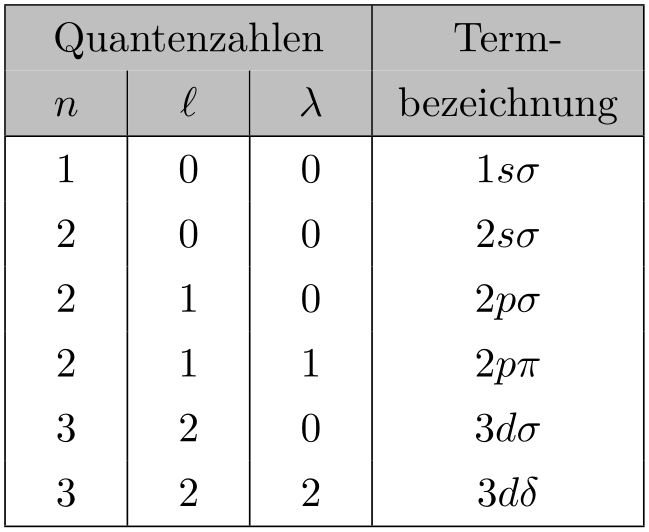
Sometimes, one wants to combine \multicolumn and \rowcolor. From what I know about LaTeX, this is a little bit complicated: it requires the use of \columncolor inside of the \multicolumn. As in the example above, it is necessary to modify the code generated by PgfplotsTable a little bit. Keep in mind that PgfplotsTable is just a code generator for tabular environments – modify whatever you want. The following example demonstrates the combination of \multicolumn and \rowcolor. It has been taken out of an – admittedly advanced – application:
\newcolumntype{C}{>{\centering\arraybackslash}p{6mm}}% a centered fixed-width-column
\pgfplotstabletypeset[
col sep=&,
row sep=\\,
every head row/.style={
% as in the previous example, this patches the first row:
before row={
\hline
\rowcolor{lightgray}
\multicolumn{3}{|>{\columncolor{lightgray}}c|}{Quantenzahlen} & Term-\\
\rowcolor{lightgray}
},
after row=\hline,
},
every last row/.style={
after row=\hline},
% define column-specific styles:
columns/n/.style={column type=|C,column name=$n$},
columns/l/.style={column type=|C,column name=$\ell$},
columns/lambda/.style={column type=|C,column name=$\lambda$},
columns/text/.style={column type=|c|,column name=bezeichnung,
string type % <-it contains formatted data
},
] {
n & l & lambda & text\\
1 & 0 & 0 & $1 s\sigma$ \\
2 & 0 & 0 & $2 s\sigma$ \\
2 & 1 & 0 & $2 p\sigma$ \\
2 & 1 & 1 & $2 p \pi $\\
3 & 2 & 0 & $3 d\sigma$ \\
3 & 2 & 2 & $3 d\delta$ \\
}
Up to the number formatting (which actually invokes \pgfmathprintnumber), the code above is equivalent to the listing
\newcolumntype{C}{>{\centering\arraybackslash}p{6mm}}% a centered fixed-width-column
\begin{tabular}{|C|C|C|c|}
\hline
\rowcolor{lightgray} \multicolumn{3}{|>{\columncolor{lightgray}}c|}{Quantenzahlen} & Term-\\
                    \rowcolor{lightgray} $n$ & $\ell$ & $\lambda$ &
                    bezeichnung\\
\hline
$1$ & $0$ & $0$ & $1 s\sigma$ \\
$2$ & $0$ & $0$ & $2 s\sigma$ \\
$2$ & $1$ & $0$ & $2 p\sigma$ \\
$2$ & $1$ & $1$ & $2 p \pi$ \\
$3$ & $2$ & $0$ & $3 d\sigma$ \\
$3$ & $2$ & $2$ & $3 d\delta$ \\
\hline
\end{tabular}
Clearly, the overhead introduced by defining a lot of styles is only worth the effort if you require number printing, automated processing, or have a huge bulk of similar tables.
-
/pgfplots/table/after row={
 TeX
code
 }
}
Contains TeX code which will be installed after the last cell in a row (i.e. after \\).
-
/pgfplots/table/every even row(style, no value) 
A style which is installed for each row with even row index. The first row is supposed to be a “head” row and does not count. Indexing starts with \(0\).
\pgfplotstableset{
columns={dof,error1,{grad(log(dof),log(error2))}},
columns/error1/.style={
column name=$L_2$,
sci,sci zerofill,sci subscript,
precision=3},
columns/dof/.style={
int detect,
column name=\textsc{Dof}},
columns/{grad(log(dof),log(error2))}/.style={
column name=slopes $L_2$,
fixed,fixed zerofill,
precision=1}}

% requires \usepackage{booktabs}
\pgfplotstabletypeset[
every head row/.style={
before row=\toprule,after row=\midrule},
every last row/.style={
after row=\bottomrule},
]
{pgfplotstable.example1.dat}
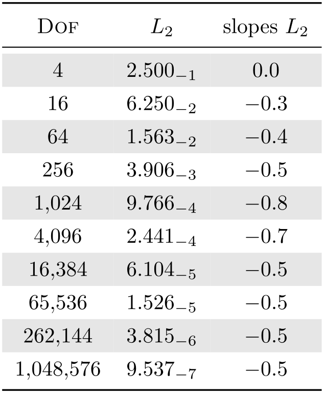
% requires \usepackage{booktabs,colortbl}
\pgfplotstabletypeset[
every even row/.style={
before row={\rowcolor[gray]{0.9}}},
every head row/.style={
before row=\toprule,after row=\midrule},
every last row/.style={
after row=\bottomrule},
]
{pgfplotstable.example1.dat}
-
/pgfplots/table/every odd row(style, no value) 
A style which is installed for each row with odd row index. The first row is supposed to be a “head” row and does not count. Indexing starts with \(0\).
-
/pgfplots/table/every head row(style, no value) 
A style which is installed for each first row in the tabular. This can be used to adjust options for column names or to add extra lines/colors.

\pgfplotstabletypeset[
% suppress the header row 'col1 col2 col3':
every head row/.style={output empty row},
col sep=comma,
columns/col1/.style={string type,column type=r},
columns/col2/.style={string type,column type=l},
columns/col3/.style={string type,column type=l},
]
{
col1,col2,col3
Col A,B,C
The first column,E,F
}
-
/pgfplots/table/every first row(style, no value) 
A style which is installed for each first data row, i.e. after the head row.
-
/pgfplots/table/every last row(style, no value) 
-
/pgfplots/table/every row no
 index
index (style, no value)
-
/pgfplots/table/every nth row={
 integer
 }{
}{ options
 }
}
-
/pgfplots/table/every nth row={
 integer[
 shift
shift ]
] }{
}{ options
 }
}
This allows to install
 options
 for every \(n\)th row with \(n=\)
 integer
 .
.

\pgfplotstabletypeset[
every nth row={3}{before row=\midrule},
every head row/.style={
before row=\toprule,after row=\midrule},
every last row/.style={
after row=\bottomrule},
]{
a b
0 0
1 1
2 2
3 3
4 4
5 5
6 6
7 7
8 8
}
Only data rows are considered for every nth row; it will never apply to column names and data rows are numbered like \(i=0,1,2,\dotsc \) (the example above applies it to the rows with \(a = 3,6\)). Since the case \(i=0\) can be handled by every first row, it is not considered for every nth row.
The second syntax allows to provide an additional
 shift
shift :
:

\pgfplotstabletypeset[
every nth row={3[+1]}{before row=\midrule},
]{
a b
0 0
1 1
2 2
3 3
4 4
5 5
6 6
7 7
8 8
9 9
10 10
}
Here, the style is applied to rows \(i=1,4,7,10\) (mathematically, it is applied if \((i \mod n) = \) shift
shift ). The
 shift
shift can be negative.
You can define many
every nth row styles, they are processed
in the order of occurrence (consider using
before row/.add={ before existing
 }{
}{ after existing
 } to modify an existing value).
Note that every nth row/.style 2 args=... is the same as every nth row=....
-
/pgfplots/table/output empty row(style, no value) 
A style which suppresses output for the current row.
This style is evaluated very late, after all column-specific content modifications have been applied. It is equivalent to
See every head row for an application.
6.1.4Configuring Single Cell Appearance: Styles
Besides the possibilities to change column styles and row styles, there are also a couple of styles to change single cells.
-
/pgfplots/table/every row
 rowindex
 column
 colindex
 (style, no value)
A style which applies to at most one cell: the one with row index
 rowindex
 and column index
 colindex
 . Each of these indices starts with \(0\).
The style is evaluated in the same context as the preproc cell content, assign cell content, and postproc cell content keys and it is a legitimate possibility to modify any of these parameters. It is also possible to replace the initial cell value by assigning something to @cell content.
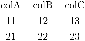
For example, consider this unmodified table:
\pgfplotstabletypeset[
col sep=&,row sep=\\]{
colA & colB & colC \\
11 & 12 & 13 \\
21 & 22 & 23 \\
}
Now, we change the number format of one of its cells, and at the same time we change the formatting of another (single) cell:
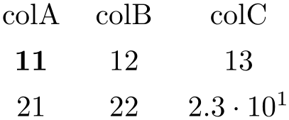
\pgfplotstabletypeset[
every row 1 column 2/.style={/pgf/number format/sci},
every row 0 column 0/.style={postproc cell content/.style={@cell content=\textbf{##1}}},
col sep=&,row sep=\\]{
colA & colB & colC \\
11 & 12 & 13 \\
21 & 22 & 23 \\
}
Note that this style is (only) applied to input row/column values.
-
/pgfplots/table/every row no
 rowindex
 column no
 colindex
 (style, no value)
This is actually the same – row no and row are both supported, the same for column and column no.
-
/pgfplots/table/every row
 rowindex
 column
 colname
 (style, no value)
A similar style as above, but it allows column names rather than column indices. Column
names need to be provided in the same way as for other column-specific styles (including the extra curly braces in case
 colname
 contains special characters).
Our example from above can thus become:
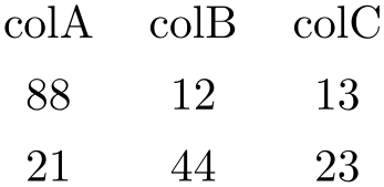
\pgfplotstabletypeset[
every row 1 column colB/.style={string replace*={2}{4}},
every row 0 column colA/.style={preproc/expr={##1*8}},
col sep=&,row sep=\\]{
colA & colB & colC \\
11 & 12 & 13 \\
21 & 22 & 23 \\
}
The example employs the string replace* preprocessor style and the preproc/expr style. All preprocessor or postprocessor styles can be used.
Please refer to Section 6.2 for predefined choices.
6.1.5Customizing and Getting the Tabular Code
The following keys allow changes of alignment (begin table) and font and they allow to write the generated code to outfiles (see also write to macro). Furthermore, the generated code can be fine–tuned to provide other sorts of table output, beyond LaTeX.
-
/pgfplots/table/every table={
 file name
 }
}
A style which is installed at the beginning of every \pgfplotstabletypeset command.103
The table file name is given as first argument.
-
/pgfplots/table/font={
 font name
 } (initially empty)
-
/pgfplots/table/begin table={
 code
code } (initially \begin{tabular})
Contains { code
code } which is generated as table start.
The following example uses a longtable instead of tabular:
Note that longtable allows the use of replicated headers for multi-page tables by means of its \endhead macro:
% replicate column names on top of every page of a multi-page table:
\pgfplotstableset{
row sep=\\,
begin table=\begin{longtable},
end table=\end{longtable},
every head row/.append style={after row=\endhead},
}
If the first page should have a different header, you can use \endfirsthead provided by the longtable package:
% replicate column names on top of every page of a multi-page table,
% but with different values for first page:
\pgfplotstableset{
row sep=\\,
begin table=\begin{longtable},
end table=\end{longtable},
every head row/.append style={after row={%
\caption{The caption}%
\endfirsthead
                                \multicolumn{3}{c}{{\bfseries \tablename\ \thetable{} --
                    continued from previous page}} \\
\endhead
},
},
}
The preceding example uses the longtable macros \caption, \endfirsthead, \thetable, and \endhead. In addition, it requires to provide the number of columns ({3} in this case) explicitly.
It is also possible to change the value of begin table. For example,
prepends the empty string {} and appends the prefix [t]. Thus, ‘\begin{tabular}’ becomes ‘\begin{tabular}[t]’.
-
/pgfplots/table/end table={
 code
code } (initially \end{tabular})
A code key which assigns /pgfplots/table/@cell content to the final output of the current cell.
The first argument, #1, is the final cell’s value. After this macro, the value of @cell content will be written to the output.
The default implementation is
/pgfplots/table/typeset cell/.code={%
\ifnum\c@pgfplotstable@colindex=\c@pgfplotstable@numcols\relax
\pgfkeyssetvalue{/pgfplots/table/@cell content}{#1\\}%
\else
\pgfkeyssetvalue{/pgfplots/table/@cell content}{#1&}%
\fi
},
The value of \pgfplotstablecol starts with \(1\) in this context, i.e. it is in the range \(1,\dotsc ,n\) where \(n=\) \pgfplotstablecols. This simplifies checks whether we have the last column.
-
/pgfplots/table/outfile={
 file name
 } (initially empty)
Writes the generated tabular code into
 file name
 . It can then be used with \input{
 file name
 }, PgfplotsTable is no longer required since it contains a completely normal
tabular.
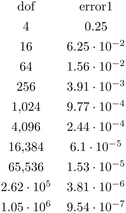
\pgfplotstabletypeset[
columns={dof,error1},
outfile=pgfplotstable.example1.out.tex]
{pgfplotstable.example1.dat}
and pgfplotstable.example1.out.tex contains
\begin {tabular}{cc}%
dof&error1\\%
\pgfutilensuremath {4}&\pgfutilensuremath {0.25}\\%
\pgfutilensuremath {16}&\pgfutilensuremath {6.25\cdot 10^{-2}}\\%
\pgfutilensuremath {64}&\pgfutilensuremath {1.56\cdot 10^{-2}}\\%
\pgfutilensuremath {256}&\pgfutilensuremath {3.91\cdot 10^{-3}}\\%
\pgfutilensuremath {1{,}024}&\pgfutilensuremath {9.77\cdot 10^{-4}}\\%
\pgfutilensuremath {4{,}096}&\pgfutilensuremath {2.44\cdot 10^{-4}}\\%
\pgfutilensuremath {16{,}384}&\pgfutilensuremath {6.1\cdot 10^{-5}}\\%
\pgfutilensuremath {65{,}536}&\pgfutilensuremath {1.53\cdot 10^{-5}}\\%
\pgfutilensuremath {2.62\cdot 10^{5}}&\pgfutilensuremath {3.81\cdot 10^{-6}}\\%
\pgfutilensuremath {1.05\cdot 10^{6}}&\pgfutilensuremath {9.54\cdot 10^{-7}}\\%
\end {tabular}%
The command \pgfutilensuremath checks whether math mode is active and switches to math mode if necessary.104
-
/pgfplots/table/include outfiles={
 boolean
 } (initially false)
If enabled, any already existing outfile will be \input instead of overwritten.
\pgfplotstableset{include outfiles} % for example in the document's preamble
This allows to place any corrections manually into generated output files since PgfplotsTable won’t overwrite the resulting tables automatically.
This will affect tables for which the outfile option is set. If you wish to apply it to every table, consider
\pgfplotstableset{every table/.append style={outfile={#1.out}}}
which will generate an outfile name for every table.
-
/pgfplots/table/force remake={
 boolean
 } (initially false)
If enabled, the effect of
include outfiles is disabled. As all
key settings only last until the next brace (or \end
 ), this key can be used to regenerate some output files while others are still included.
-
/pgfplots/table/write to macro={
 \macroname
 }
}
If the value of
write to macro is not empty, the
completely generated (tabular) code will be written into the macro
 \macroname
 .
.
See the typeset=false key in case you need only the resulting macro.
-
/pgfplots/table/skip coltypes=true|false (initially false) 
Allows to skip the
 coltypes
 in \begin{tabular}{
 coltypes
 }. This allows simplifications for other table types which don’t have
LaTeX’s table format.
-
/pgfplots/table/typeset=true|false (initially true) 
A boolean which disables the final typesetting stage. Use typeset=false in conjunction with write to macro if only the generated code is of interest and TeX should not attempt to produce any content in the output pdf.
-
/pgfplots/table/debug={
 boolean
 } (initially false)
If enabled, it will write every final tabular code to your logfile.
-
/pgfplots/table/TeX comment={
 comment sign
 } (initially %)
The comment sign which is inserted into outfiles to suppress trailing white space.
As a last example, we use PgfplotsTable to write an .html file (including number formatting and rounding!):

\pgfplotstabletypeset[
begin table={}, end table={
typeset cell/.style={
/pgfplots/table/@cell content={#1}
},
before row=,after row=,
skip coltypes, typeset=false,
verbatim,% configures number printer
TeX comment=,
columns={level,dof,error1},
outfile=pgfplotstable.example1.out.html,
]{pgfplotstable.example1.dat}
\lstinputlisting
[basicstyle=\ttfamily\footnotesize]
{pgfplotstable.example1.out.html}
103 The every table style is installed after options provided to \pgfplotstabletypeset; it has higher precedence.
104 Please note that \pgfutilensuremath needs to be replaced by \ensuremath if you want to use the output file independent of pgf. That can be done by \let\pgfutilensuremath=\ensuremath which enables the LaTeX command \ensuremath.
6.1.6Defining Column Types for tabular
Besides input of text files, it is sometimes desirable to define column types for existing tabular environments.
-
\newcolumntype{
 letter
 }[
}[ number of arguments
 ]\(>\){
 before column
 }
} column type
 \(<\){
 after column
 }
}
The command
\newcolumntype is part of the
array package and it defines a new column type
 letter
 for use in
LaTeX
tabular environments.
\usepackage{array}
Now, the environment pgfplotstablecoltype can be used in
 before column
 and
and
 after column
 to define numerical columns:
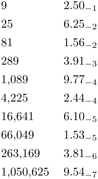
% requires \usepackage{array}
\newcolumntype{L}[1]
{>{\begin{pgfplotstablecoltype}[#1]}r<{\end{pgfplotstablecoltype}}}
\begin{tabular}{L{int detect}L{sci,sci subscript,sci zerofill}}
9 & 2.50000000e-01\\
25 & 6.25000000e-02\\
81 & 1.56250000e-02\\
289 & 3.90625000e-03\\
1089 & 9.76562500e-04\\
4225 & 2.44140625e-04\\
16641 & 6.10351562e-05\\
66049 & 1.52587891e-05\\
263169 & 3.81469727e-06\\
1050625& 9.53674316e-07\\
\end{tabular}
The environment pgfplotstablecoltype accepts an optional argument which may contain any number formatting options. It is an error if numerical columns contain non-numerical data, so it may be necessary to use \multicolumn for column names.
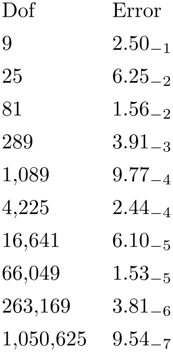
% requires \usepackage{array}
\newcolumntype{L}[1]
{>{\begin{pgfplotstablecoltype}[#1]}r<{\end{pgfplotstablecoltype}}}
\begin{tabular}{L{int detect}L{sci,sci subscript,sci zerofill}}
\multicolumn{1}{r}{Dof} & \multicolumn{1}{r}{Error}\\
9 & 2.50000000e-01\\
25 & 6.25000000e-02\\
81 & 1.56250000e-02\\
289 & 3.90625000e-03\\
1089 & 9.76562500e-04\\
4225 & 2.44140625e-04\\
16641 & 6.10351562e-05\\
66049 & 1.52587891e-05\\
263169 & 3.81469727e-06\\
1050625& 9.53674316e-07\\
\end{tabular}
6.1.7Number Formatting Options
The following extract of the PGF/TikZ manual explains how to configure number formats. The common option prefix /pgf/number format can be omitted; it will be recognized automatically.
All these number formatting options can also be applied to pgfplots.
-
\pgfmathprintnumber{
 x
x }
}
Generates pretty-printed output for the (real) number
 x
x . The input number
 x
x is parsed using \pgfmathfloatparsenumber which allows arbitrary precision.
Numbers are typeset in math mode using the current set of number printing options, see below. Optional arguments can also be
provided using \pgfmathprintnumber[ options
 ]{
]{ x
x }.
}.
-
\pgfmathprintnumberto{
 x
x }{
}{ \macro
 }
}
Returns the resulting number into
 \macro
 instead of typesetting it directly.
-
/pgf/number format/fixed(no value) 
Configures \pgfmathprintnumber to round the number to a fixed number of digits after the period, discarding any trailing zeros.

\pgfkeys{/pgf/number format/.cd,fixed,precision=2}
\pgfmathprintnumber{4.568}\hspace{1em}
\pgfmathprintnumber{5e-04}\hspace{1em}
\pgfmathprintnumber{0.1}\hspace{1em}
\pgfmathprintnumber{24415.98123}\hspace{1em}
\pgfmathprintnumber{123456.12345}
See Section 6.1.7.1 for how to change the appearance.
-
/pgf/number format/fixed zerofill={
 boolean
 }
(default true)
Enables or disables zero filling for any number drawn in fixed point format.

\pgfkeys{/pgf/number format/.cd,fixed,fixed zerofill,precision=2}
\pgfmathprintnumber{4.568}\hspace{1em}
\pgfmathprintnumber{5e-04}\hspace{1em}
\pgfmathprintnumber{0.1}\hspace{1em}
\pgfmathprintnumber{24415.98123}\hspace{1em}
\pgfmathprintnumber{123456.12345}
This key affects numbers drawn with fixed or std styles (the latter only if no scientific format is chosen).

\pgfkeys{/pgf/number format/.cd,std,fixed zerofill,precision=2}
\pgfmathprintnumber{4.568}\hspace{1em}
\pgfmathprintnumber{5e-05}\hspace{1em}
\pgfmathprintnumber{1}\hspace{1em}
\pgfmathprintnumber{123456.12345}
See Section 6.1.7.1 for how to change the appearance.
-
/pgf/number format/sci(no value) 
Configures \pgfmathprintnumber to display numbers in scientific format, that means sign, mantissa and exponent (base \(10\)). The mantissa is rounded to the desired precision (or sci precision, see below).

\pgfkeys{/pgf/number format/.cd,sci,precision=2}
\pgfmathprintnumber{4.568}\hspace{1em}
\pgfmathprintnumber{5e-04}\hspace{1em}
\pgfmathprintnumber{0.1}\hspace{1em}
\pgfmathprintnumber{24415.98123}\hspace{1em}
\pgfmathprintnumber{123456.12345}
See Section 6.1.7.1 for how to change the exponential display style.
-
/pgf/number format/sci zerofill={
 boolean
 }
(default true)
Enables or disables zero filling for any number drawn in scientific format.

\pgfkeys{/pgf/number format/.cd,sci,sci zerofill,precision=2}
\pgfmathprintnumber{4.568}\hspace{1em}
\pgfmathprintnumber{5e-04}\hspace{1em}
\pgfmathprintnumber{0.1}\hspace{1em}
\pgfmathprintnumber{24415.98123}\hspace{1em}
\pgfmathprintnumber{123456.12345}
As with fixed zerofill, this option does only affect numbers drawn in sci format (or std if the scientific format is chosen).
See Section 6.1.7.1 for how to change the exponential display style.
-
/pgf/number format/zerofill={
 boolean
 }
(style, default true)
-
/pgf/number format/std(no value) 
-
/pgf/number format/std=
 lower e
-
/pgf/number format/std=
 lower e
 :
: upper e
Configures \pgfmathprintnumber to a standard algorithm. It chooses either fixed or sci, depending on the order of magnitude. Let \(n=s \cdot m \cdot 10^e\) be the input number and \(p\) the current precision. If \(-p/2 \le e \le 4\), the number is displayed using fixed format. Otherwise, it is displayed using sci format.

\pgfkeys{/pgf/number format/.cd,std,precision=2}
\pgfmathprintnumber{4.568}\hspace{1em}
\pgfmathprintnumber{5e-04}\hspace{1em}
\pgfmathprintnumber{0.1}\hspace{1em}
\pgfmathprintnumber{24415.98123}\hspace{1em}
\pgfmathprintnumber{123456.12345}
The parameters can be customized using the optional integer argument(s): if
 lower e
 \(\le e \le \)
 upper e
 , the number is displayed in fixed format, otherwise in sci format. Note that
 lower e
 should be negative for useful results. The precision used for scientific format can be adjusted with
sci precision if necessary.
-
/pgf/number format/relative*=
 exponent base 10
Configures \pgfmathprintnumber to format numbers relative to an order of magnitude, \(10^r\), where \(r\) is an integer number.
This key addresses different use-cases.
provide a unified format for a sequence of numbers. Consider the following test:

\pgfkeys{/pgf/number format/relative*={1}}
\pgfmathprintnumber{6.42e-16}\hspace{1em}
\pgfmathprintnumber{1.2}\hspace{1em}
\pgfmathprintnumber{6}\hspace{1em}
\pgfmathprintnumber{20.6}\hspace{1em}
\pgfmathprintnumber{87}
With any other style, the 6.42e-16 would have been formatted as an isolated number. Here, it is rounded to 0 because when viewed relative to \(10^1\) (the exponent \(1\) is the argument for relative), it has no significant digits.

\pgfkeys{/pgf/number format/relative*={2}}
\pgfmathprintnumber{123.345}\hspace{1em}
\pgfmathprintnumber{0.0012}\hspace{1em}
\pgfmathprintnumber{0.0014}\hspace{1em}
The example above applies the initial precision=2 to 123.345 – relative to \(100\). Two significant digits of 123.345 relative to \(100\) are 123. Note that the “\(2\) significant digits of 123.345” translates to “round 1.2345 to \(2\) digits”, which would yield 1.2300. Similarly, the other two numbers are 0 compared to \(100\) using the given precision.

\pgfkeys{/pgf/number format/relative*={-3}}
\pgfmathprintnumber{123.345}\hspace{1em}
\pgfmathprintnumber{0.0012}\hspace{1em}
\pgfmathprintnumber{0.0014}\hspace{1em}
improve rounding in the presence of inaccurate numbers. Let us suppose that some limited-precision arithmetics resulted in the result 123456999 (like the fpu of pgf). You know that its precision is about five or six significant digits. And you want to provide a fixed point output. In this case, the trailing digits ....999 are a numerical artifact due to the limited precision. Use relative*=3,precision=0 to eliminate the artifacts:

\pgfkeys{/pgf/number format/.cd,relative*={3},precision=0}
\pgfmathprintnumber{123456999}\hspace{1em}
\pgfmathprintnumber{123456999.12}
Here, precision=0 means that we inspect 123456.999 and round that number to \(0\) digits. Finally, we move the period back to its initial position. Adding relative style=fixed results in fixed point output format:

\pgfkeys{/pgf/number format/.cd,relative*={3},precision=0,relative style=fixed}
\pgfmathprintnumber{123456999}\hspace{1em}
\pgfmathprintnumber{123456999.12}
Note that there is another alternative for this use-case which is discussed later: the fixed relative style.

\pgfkeys{/pgf/number format/.cd,fixed relative,precision=6}
\pgfmathprintnumber{123456999}\hspace{1em}
\pgfmathprintnumber{123456999.12}
You might wonder why there is an asterisk in the key’s name. The short answer is: there is also a /pgf/number format/relative number printer which does unexpected things. The key relative* repairs this. Existing code will still use the old behavior.
Technically, the key works as follows: as already explained above, relative*=3 key applied to 123456999.12 moves the period by three positions and analyzes 123456.99912. Mathematically speaking, we are given a number \(x = \pm m \cdot 10^e\) and we attempt to apply relative*=\(r\). The method then rounds \(x / 10^r\) to precision digits. Afterwards, it multiplies the result by \(10^r\) and typesets it.
-
/pgf/number format/every relative(style, no value) 
A style which configures how the relative method finally displays its results.
The initial configuration is
Note that rounding is turned off when the resulting style is being evaluated (since relative already rounded the number).
Although supported, I discourage from using fixed zerofill or sci zerofill in this context – it may lead to a suggestion of higher precision than is actually used (because fixed zerofill might simply add .00 although there was a different information before relative rounded the result).
-
/pgf/number format/relative style={
 options
 }
}
The same as
every relative/.append style={ options
 }.
}.
-
/pgf/number format/fixed relative(no value) 
Configures \pgfmathprintnumber to format numbers in a similar way to the fixed style, but the precision is interpreted relatively to the number’s exponent.
The motivation is to get the same rounding effect as for sci, but to display the number in the fixed style:

\pgfkeys{/pgf/number format/.cd,fixed relative,precision=3}
\pgfmathprintnumber{1000.0123}\hspace{1em}
\pgfmathprintnumber{100.0567}\hspace{1em}
\pgfmathprintnumber{0.000010003452}\hspace{1em}
\pgfmathprintnumber{0.010073452}\hspace{1em}
\pgfmathprintnumber{1.23567}\hspace{1em}
\pgfmathprintnumber{1003.75}\hspace{1em}
\pgfmathprintnumber{1006.75}\hspace{1em}
The effect of fixed relative is that the number is rounded to exactly the first
 precision
 non-zero digits, no matter how many leading zeros the number might have.
Use fixed relative if you want fixed and if you know that only the first \(n\) digits are correct. Use sci if you need a scientific display style and only the first \(n\) digits are correct.
Note that fixed relative ignores the fixed zerofill flag.
See also the relative* key. Note that the relative={ exponent
 } key explicitly moves the period to some designated position before it attempts to round the number. Afterwards, it
“rounds from the right”, i.e. it rounds to that explicitly chosen digit position. In contrast to that,
fixed relative “rounds from the left”: it takes the first non-zero digit, temporarily places
the period after this digit, and rounds that number. The rounding style fixed leaves the period where it is, and
rounds everything behind that digit. The sci style is similar to fixed relative.
-
/pgf/number format/int detect(no value) 
Configures \pgfmathprintnumber to detect integers automatically. If the input number is an integer, no period is displayed at all. If not, the scientific format is chosen.

\pgfkeys{/pgf/number format/.cd,int detect,precision=2}
\pgfmathprintnumber{15}\hspace{1em}
\pgfmathprintnumber{20}\hspace{1em}
\pgfmathprintnumber{20.4}\hspace{1em}
\pgfmathprintnumber{0.01}\hspace{1em}
\pgfmathprintnumber{0}
-
\pgfmathifisint{
 number constant
 }{
}{ true code
 }{
}{ false code
 }
}
A command which does the same check as int detect, but it invokes
 true code
 if the
 number constant
 actually is an integer and the
 false code
 if not.
As a side-effect, \pgfretval will contain the parsed number, either in integer format or as parsed floating point number.
The argument
 number constant
 will be parsed with \pgfmathfloatparsenumber.

                    15 \pgfmathifisint{15}{is an int: \pgfretval.}{is no
                    int}\hspace{1em}
                    15.5 \pgfmathifisint{15.5}{is an int:
                    \pgfretval.}{is no int}
-
/pgf/number format/int trunc(no value) 
Truncates every number to integers (discards any digit after the period).

\pgfkeys{/pgf/number format/.cd,int trunc}
\pgfmathprintnumber{4.568}\hspace{1em}
\pgfmathprintnumber{5e-04}\hspace{1em}
\pgfmathprintnumber{0.1}\hspace{1em}
\pgfmathprintnumber{24415.98123}\hspace{1em}
\pgfmathprintnumber{123456.12345}
-
/pgf/number format/frac(no value) 
-
/pgf/number format/frac TeX={
 \macro
 } (initially \frac)
-
/pgf/number format/frac denom=
 int
int (initially empty)
-
/pgf/number format/frac whole=true|false (initially true) 
-
/pgf/number format/frac shift={
 integer
 } (initially 4)
Displays numbers as fractionals.

\pgfkeys{/pgf/number format/frac}
\pgfmathprintnumber{0.333333333333333}\hspace{1em}
\pgfmathprintnumber{0.5}\hspace{1em}
\pgfmathprintnumber{2.133333333333325e-01}\hspace{1em}
\pgfmathprintnumber{0.12}\hspace{1em}
\pgfmathprintnumber{2.666666666666646e-02}\hspace{1em}
\pgfmathprintnumber{-1.333333333333334e-02}\hspace{1em}
\pgfmathprintnumber{7.200000000000000e-01}\hspace{1em}
\pgfmathprintnumber{6.666666666666667e-02}\hspace{1em}
\pgfmathprintnumber{1.333333333333333e-01}\hspace{1em}
\pgfmathprintnumber{-1.333333333333333e-02}\hspace{1em}
\pgfmathprintnumber{3.3333333}\hspace{1em}
\pgfmathprintnumber{1.2345}\hspace{1em}
\pgfmathprintnumber{1}\hspace{1em}
\pgfmathprintnumber{-6}
Allows to use a different implementation for \frac inside of the frac display type.
Allows to provide a custom denominator for frac.

\pgfkeys{/pgf/number format/.cd,frac, frac denom=10}
\pgfmathprintnumber{0.1}\hspace{1em}
\pgfmathprintnumber{0.5}\hspace{1em}
\pgfmathprintnumber{1.2}\hspace{1em}
\pgfmathprintnumber{-0.6}\hspace{1em}
\pgfmathprintnumber{-1.4}\hspace{1em}
Configures whether complete integer parts shall be placed in front of the fractional part. In this case, the fractional part will be less then \(1\). Use frac whole=false to avoid whole number parts.

\pgfkeys{/pgf/number format/.cd,frac, frac whole=false}
\pgfmathprintnumber{20.1}\hspace{1em}
\pgfmathprintnumber{5.5}\hspace{1em}
\pgfmathprintnumber{1.2}\hspace{1em}
\pgfmathprintnumber{-5.6}\hspace{1em}
\pgfmathprintnumber{-1.4}\hspace{1em}
In case you experience stability problems, try experimenting with a different frac shift. Higher shift values \(k\) yield higher sensitivity to inaccurate data or inaccurate arithmetics.
Technically, the following happens. If \(r < 1\) is the fractional part of the mantissa, then a scale \(i = 1/r \cdot 10^k\) is computed where \(k\) is the shift; fractional parts of \(i\) are neglected. The value \(1/r\) is computed internally, its error is amplified.
If you still experience stability problems, use \usepackage{fp} in your preamble. The frac style will then automatically employ the higher absolute precision of fp for the computation of \(1/r\).
-
/pgf/number format/precision={
 number
 }
}
Sets the desired rounding precision for any display operation. For scientific format, this affects the mantissa.
-
/pgf/number format/sci precision=
 number or empty
 (initially empty)
Sets the desired rounding precision only for sci styles.
Use sci precision={} to restore the initial configuration (which uses the argument provided to precision for all number styles).
-
/pgf/number format/read comma as period=true|false (initially false) 
This is one of the few keys which allows to customize the number parser. If this switch is turned on, a comma is read just as a period.

This is typically undesired as it can cause side-effects with math parsing instructions. However, it is supported to format input numbers or input tables. Consider use comma to typeset the result with a comma as well.

this key requires a pgf version which is more recent than pgf 3.0.0.
6.1.7.1Changing Number Format Display Styles
You can change the way how numbers are displayed. For example, if you use the ‘fixed’ style, the input number is rounded to the desired precision and the current fixed point display style is used to typeset the number. The same is applied to any other format: first, rounding routines are used to get the correct digits, afterwards a display style generates proper TeX-code.
-
/pgf/number format/set decimal separator={
 text
text }
}
Assigns
 text
text as decimal separator for any fixed point number (including the mantissa in sci format).
-
/pgf/number format/dec sep={
 text
text }
}
-
/pgf/number format/set thousands separator={
 text
text }
}
Assigns
 text
text as thousands separator for any fixed point number (including the mantissa in sci format).

\pgfkeys{/pgf/number format/.cd,
fixed,
fixed zerofill,
precision=2,
set thousands separator={}}
\pgfmathprintnumber{1234.56}

\pgfkeys{/pgf/number format/.cd,
fixed,
fixed zerofill,
precision=2,
set thousands separator={}}
\pgfmathprintnumber{1234567890}

\pgfkeys{/pgf/number format/.cd,
fixed,
fixed zerofill,
precision=2,
set thousands separator={.}}
\pgfmathprintnumber{1234567890}

\pgfkeys{/pgf/number format/.cd,
fixed,
fixed zerofill,
precision=2,
set thousands separator={,}}
\pgfmathprintnumber{1234567890}

\pgfkeys{/pgf/number format/.cd,
fixed,
fixed zerofill,
precision=2,
set thousands separator={{{{,}}}}}
\pgfmathprintnumber{1234567890}
The last example employs commas and disables the default comma-spacing.
-
/pgf/number format/1000 sep={
 text
text }
}
-
/pgf/number format/1000 sep in fractionals={
 boolean
 } (initially false)
Configures whether the fractional part should also be grouped into groups of three digits.
The value true will activate the 1000 sep for both integer and fractional parts. The value false will activate 1000 sep only for the integer part.

\pgfkeys{/pgf/number format/.cd,
fixed,
precision=999,
set thousands separator={\,},
1000 sep in fractionals,
}
\pgfmathprintnumber{1234.1234567}

\pgfkeys{/pgf/number format/.cd,
fixed,fixed zerofill,
precision=9,
set thousands separator={\,},
1000 sep in fractionals,
}
\pgfmathprintnumber{1234.1234567}
-
/pgf/number format/min exponent for 1000 sep={
 number
 } (initially 0)
Defines the smallest exponent in scientific notation which is required to draw thousand separators. The exponent is the number of digits minus one, so \(\meta {number}=4\) will use thousand separators starting with \(1e4 = 10000\).

\pgfkeys{/pgf/number format/.cd,
int detect,
1000 sep={\,},
min exponent for 1000 sep=0}
\pgfmathprintnumber{5000}; \pgfmathprintnumber{1000000}

\pgfkeys{/pgf/number format/.cd,
int detect,
1000 sep={\,},
min exponent for 1000 sep=4}
\pgfmathprintnumber{1000}; \pgfmathprintnumber{5000}

\pgfkeys{/pgf/number format/.cd,
int detect,
1000 sep={\,},
min exponent for 1000 sep=4}
\pgfmathprintnumber{10000}; \pgfmathprintnumber{1000000}
A value of 0 disables this feature (negative values are ignored).
-
/pgf/number format/use period(no value) 
A predefined style which installs periods ‘.’ as decimal separators and commas ‘,’ as thousands separators. This style is the default.

\pgfkeys{/pgf/number format/.cd,fixed,precision=2,use period}
\pgfmathprintnumber{12.3456}

\pgfkeys{/pgf/number format/.cd,fixed,precision=2,use period}
\pgfmathprintnumber{1234.56}
-
/pgf/number format/use comma(no value) 
A predefined style which installs commas ‘,’ as decimal separators and periods ‘.’ as thousands separators.

\pgfkeys{/pgf/number format/.cd,fixed,precision=2,use comma}
\pgfmathprintnumber{12.3456}

\pgfkeys{/pgf/number format/.cd,fixed,precision=2,use comma}
\pgfmathprintnumber{1234.56}
-
/pgf/number format/skip 0.={
 boolean
 } (initially false)
Configures whether numbers like \(0.1\) shall be typeset as \(.1\) or not.

\pgfkeys{/pgf/number format/.cd,
fixed,
fixed zerofill,precision=2,
skip 0.}
\pgfmathprintnumber{0.56}

\pgfkeys{/pgf/number format/.cd,
fixed,
fixed zerofill,precision=2,
skip 0.=false}
\pgfmathprintnumber{0.56}
-
/pgf/number format/showpos={
 boolean
 } (initially false)
Enables or disables display of plus signs for non-negative numbers.


\pgfkeys{/pgf/number format/showpos=false}
\pgfmathprintnumber{12.345}

\pgfkeys{/pgf/number format/.cd,showpos,sci}
\pgfmathprintnumber{12.345}
-
/pgf/number format/print sign={
 boolean
 }
}
-
/pgf/number format/sci 10e(no value) 
Uses \(m \cdot 10^e\) for any number displayed in scientific format.

\pgfkeys{/pgf/number format/.cd,sci,sci 10e}
\pgfmathprintnumber{12.345}
-
/pgf/number format/sci 10^e(no value) 
-
/pgf/number format/sci e(no value) 
Uses the ‘\(1e{+}0\)’ format which is generated by common scientific tools for any number displayed in scientific format.

\pgfkeys{/pgf/number format/.cd,sci,sci e}
\pgfmathprintnumber{12.345}
-
/pgf/number format/sci E(no value) 
The same with an uppercase ‘E’.

\pgfkeys{/pgf/number format/.cd,sci,sci E}
\pgfmathprintnumber{12.345}
-
/pgf/number format/sci subscript(no value) 
Typesets the exponent as subscript for any number displayed in scientific format. This style requires very little space.

\pgfkeys{/pgf/number format/.cd,sci,sci subscript}
\pgfmathprintnumber{12.345}
-
/pgf/number format/sci superscript(no value) 
Typesets the exponent as superscript for any number displayed in scientific format. This style requires very little space.

\pgfkeys{/pgf/number format/.cd,sci,sci superscript}
\pgfmathprintnumber{12.345}
-
/pgf/number format/sci generic={
 keys
keys }
}
-
/pgf/number format/sci generic/mantissa sep={
 text
text } (initially empty)
-
/pgf/number format/sci generic/exponent={
 text
text } (initially empty)
Allows to define a
custom number style for the scientific format. Here,
 keys
keys can be one of the following choices (omit the long key prefix):
Provides the separator between the mantissa and the exponent. It might be \cdot, for example,
Provides text to format the exponent. The actual exponent is available as argument #1 (see below).

\pgfkeys{
/pgf/number format/.cd,
sci,
sci generic={mantissa sep=\times,exponent={10^{#1}}}}
\pgfmathprintnumber{12.345};
\pgfmathprintnumber{0.00012345}
The
 keys
keys can depend on three parameters, namely on #1 which is the exponent, #2 containing the flags entity of
the floating point number and #3 is the (unprocessed and unformatted) mantissa.
Note that sci generic is not suitable to modify the appearance of fixed point numbers, nor can it be used to format the mantissa (which is typeset like fixed point numbers). Use dec sep, 1000 sep and print sign to customize the mantissa.
-
/pgf/number format/retain unit mantissa=true|false (initially true) 
Allows to omit a unit mantissa.

\pgfkeys{
/pgf/number format/.cd,
sci, retain unit mantissa=false}
\pgfmathprintnumber{10.5};
\pgfmathprintnumber{10};
\pgfmathprintnumber{1010};
\pgfmathprintnumber[precision=1]{-1010};
The feature is applied after rounding to the desired precision: if the remaining mantissa is equal to \(1\), it will be omitted. It applies to all styles involving the scientific format (including std).
-
/pgf/number format/@dec sep mark={
 text
text }
}
Will be placed right
before the place where a decimal separator belongs to. However,
 text
text will be inserted even if there is no decimal separator. It is intended as place-holder for auxiliary routines to find
alignment positions.
This key should never be used to change the decimal separator! Use dec sep instead.
-
/pgf/number format/@sci exponent mark={
 text
text }
}
Will be placed right before exponents in scientific notation. It is intended as place-holder for auxiliary routines to find alignment positions.
This key should never be used to change the exponent!
-
/pgf/number format/assume math mode={
 boolean
 }
(default true)
Set this to true if you don’t want any checks for math mode.
The initial setting installs a \pgfutilensuremath around each final number to change to math mode if necessary. Use assume math mode=true if you know that math mode is active and you don’t want \pgfutilensuremath.
-
/pgf/number format/verbatim(style, no value) 
A style which configures the number printer to produce verbatim text output, i.e. it doesn’t contain TeX macros.

\pgfkeys{
/pgf/fpu,
/pgf/number format/.cd,
sci,
verbatim}
\pgfmathprintnumber{12.345};
\pgfmathprintnumber{0.00012345};
\pgfmathparse{exp(15)}
\pgfmathprintnumber{\pgfmathresult}
The style resets 1000 sep, dec sep, print sign, skip 0. and sets assume math mode. Furthermore, it installs a sci generic format for verbatim output of scientific numbers.
However, it will still respect precision, fixed zerofill, sci zerofill and the overall styles fixed, sci, int detect (and their variants). It might be useful if you intend to write output files.