Manual for Package pgfplots
2D/3D Plots in LATeX, Version 1.18.2
https://github.com/pgf-tikz/pgfplots
The Reference
4.7Markers, Linestyles, (Background) Colors and Colormaps
The following options of TikZ are available to plots.
4.7.1Markers
This list is copied from the PGF/TikZ manual (Section 29).
-
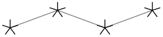
mark=*
-
mark=x

-
mark=+
And with \usetikzlibrary{plotmarks}:
-
mark=\(-\)

-
mark=\(\vert \)
-
mark=o

-
mark=asterisk
-
mark=star
-
mark=10-pointed star

-
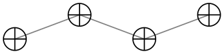
mark=oplus
-
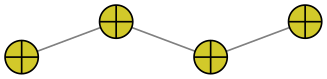
mark=oplus*
-
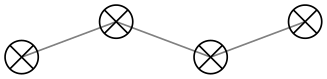
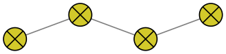
mark=otimes
-
mark=otimes*
-
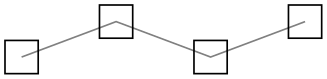
mark=square
-
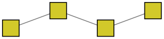
mark=square*
-
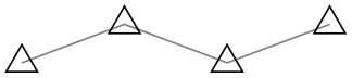
mark=triangle
-
mark=triangle*
-
mark=diamond
-
mark=diamond*
-
mark=halfdiamond*
-
mark=halfsquare*
-
mark=halfsquare right*
-
mark=halfsquare left*
-
mark=Mercedes star
-
mark=Mercedes star flipped
-
mark=halfcircle
One half is filled with white (more precisely, with mark color).
-
mark=halfcircle*
One half is filled with white (more precisely, with mark color) and the other half is filled with the actual fill color.
-
mark=pentagon
-
mark=pentagon*

-
mark=ball
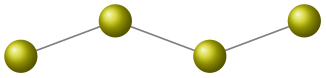
This marker is special and can easily generate big output files if there are lots of them. It is also special in that it needs ball color to be set (in our case, it is ball color=yellow!80!black.
-
mark=text

This marker is special as it can be configured freely. The character (or even text) used is configured by a set of variables, see below.
-
mark=cube
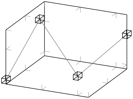
This marker is only available inside of a pgfplots axis, it draws a cube with axis parallel faces. Its dimensions can be configured separately, see below.
-
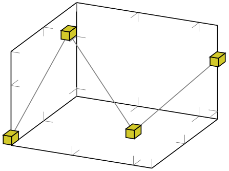
mark=cube*
-
User defined It is possible to define new markers with \pgfdeclareplotmark, see below.
All these options have been drawn with the additional options
Please see Section 4.7.5 for how to change draw and fill colors. Note that each of the provided marks can be rotated freely by means of mark options={rotate=90} or every mark/.append style={rotate=90}.
-
/tikz/mark size={
 dimension
 } (initially 2pt)
} (initially 2pt)
This TikZ option allows to set
marker sizes to
dimension. For circular markers,
dimension
is the radius, for other plot marks it is about half the width and height.
-
/tikz/every mark(no value) 
This TikZ style can be reconfigured to set marker appearance options like colors or transformations like scaling or rotation. pgfplots appends its cycle list options to this style.
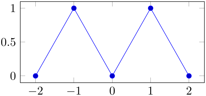
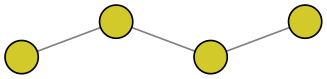
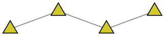
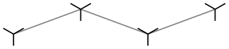
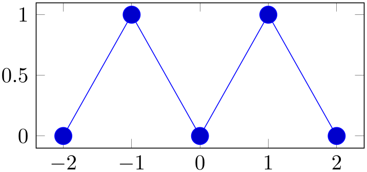
% Preamble: \pgfplotsset{width=7cm,compat=1.18}
\begin{tikzpicture}
\begin{axis}[y=2cm]
\addplot coordinates
{(-2,0) (-1,1) (0,0) (1,1) (2,0)};
\end{axis}
\end{tikzpicture}
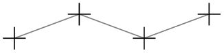
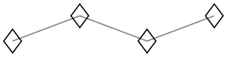
% Preamble: \pgfplotsset{width=7cm,compat=1.18}
\tikzset{every mark/.append style={scale=2}}
\begin{tikzpicture}
\begin{axis}[y=2cm]
\addplot coordinates
{(-2,0) (-1,1) (0,0) (1,1) (2,0)};
\end{axis}
\end{tikzpicture}
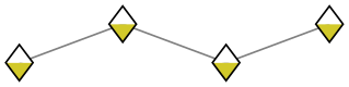
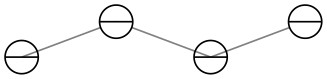
% Preamble: \pgfplotsset{width=7cm,compat=1.18}
\begin{tikzpicture}
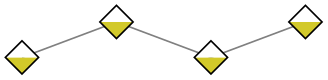
\begin{axis}[y=2cm]
\addplot+ [
mark=halfcircle*,
every mark/.append style={rotate=90}]
coordinates
{(-2,0) (-1,1) (0,0) (1,1) (2,0)};
\addplot+ [
mark=halfcircle*,
every mark/.append style={rotate=180}]
coordinates
{(-2,-0.1) (-1,0.9) (0,-0.1) (1,0.9) (2,-0.1)};
\end{axis}
\end{tikzpicture}
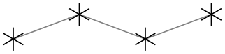
Note that every mark is kind of static in the sense that it is evaluated once only. If you need individually colored marks as part of a scatter plot, you will need to resort to scatter/use mapped color.
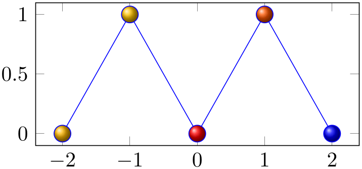
% Preamble: \pgfplotsset{width=7cm,compat=1.18}
\begin{tikzpicture}
\begin{axis}[y=2cm]
\addplot+ [
mark=ball,
mark size=4pt,
                            scatter,%
                    enable scatter
scatter src=rand,% the "color data"
% configure individual appearances:
scatter/use mapped color=
{ball color=mapped color}]
coordinates
{(-2,0) (-1,1) (0,0) (1,1) (2,0)};
\end{axis}
\end{tikzpicture}
-
/pgfplots/no markers(style, no value) 
A key which overrides any mark value set by cycle list of option lists after \addplot.
If this style is provided as argument to a complete axis, it is appended to every axis plot post such that it disables markers even for cycle lists which contain markers.
-
/tikz/mark phase={
integer \(p\)} (initially 1)
This option allows to control which markers are drawn. It is primarily used together with the TikZ option mark repeat=\(r\): it tells TikZ that the first mark to be drawn should be the \(p\)th, followed by the \((p + r)\)th, then the \((p + 2r)\)th, and so on.
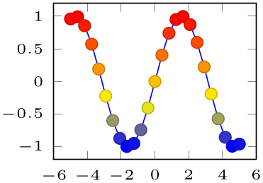
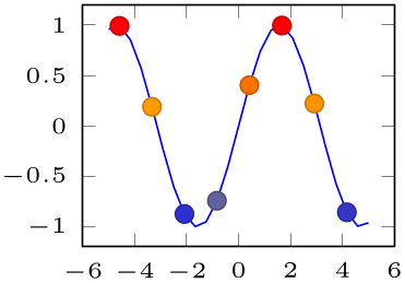
% Preamble: \pgfplotsset{width=7cm,compat=1.18}
\begin{tikzpicture}
\begin{axis}[tiny]
                            \addplot+
                    [scatter] {sin(deg(x))};
\end{axis}
\end{tikzpicture}
\begin{tikzpicture}
\begin{axis}[tiny]
                            \addplot+
                    [scatter,
mark repeat=3,mark phase=2]
{sin(deg(x))};
\end{axis}
\end{tikzpicture}
Here, \(p=1\) is the first point (the one with \coordindex\(=0\)).
-
/tikz/mark indices={
index list} (initially empty)
Allows to draw only the marker whose index numbers are in the argument list.
-
/pgf/mark color={
color} (initially empty)
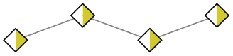
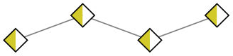
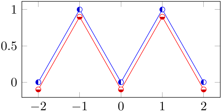
Defines the additional fill color for the halfcircle, halfcircle*, halfdiamond* and halfsquare* markers. An empty value uses white (which is the initial configuration). The value none disables filling for this part.
These markers have two distinct fill colors, one is determined by fill as for any other marker and the other one is mark color.
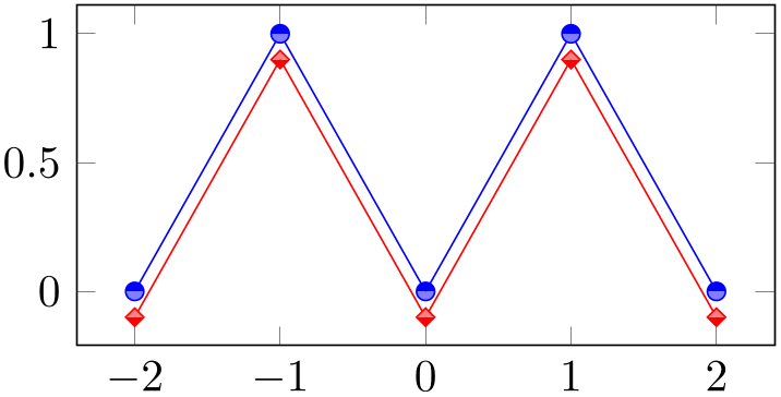
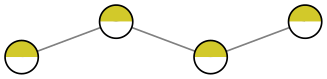
% Preamble: \pgfplotsset{width=7cm,compat=1.18}
\begin{tikzpicture}
\begin{axis}[y=2cm]
\addplot [
blue,
mark color=blue!50!white,
mark=halfcircle*
] coordinates {
(-2,0) (-1,1) (0,0) (1,1) (2,0)
};
\addplot [
red,
mark color=red!50!white,
mark=halfsquare*,
] coordinates {
(-2,-0.1) (-1,0.9) (0,-0.1) (1,0.9) (2,-0.1)
};
\end{axis}
\end{tikzpicture}
Note that this key requires pgf 2.10 or later.
-
/tikz/mark options={
options}
Resets
every mark to {options}.
-
/pgf/text mark={
text} (initially p)
Changes the text shown by mark=text.
With /pgf/text mark=m:

With /pgf/text mark=A:

There is no limitation about the number of characters or whatever. In fact, any
TeX
material can be inserted as
text, including images.
-
/pgf/text mark style={
options for mark=text}
Defines a set of options which control the appearance of mark=text.
If /pgf/text mark as node=false (the default),
options
is provided as argument to \pgftext – which provides only some basic keys like left,
right, top, bottom, base and rotate.
If /pgf/text mark as node=true,
options
is provided as argument to \node. This means you can provide a very powerful set of options including
anchor, scale, fill, draw, rounded corners, etc.
-
\pgfdeclareplotmark{
plot mark name}{code}
Defines a new marker named
plot mark name. Whenever it is used,
code
will be invoked. It is supposed to contain (preferable pgf basic level) drawing commands. During
code, the coordinate system’s origin denotes the coordinate where the marker shall be placed.
Please refer to the PGF/TikZ manual section “Mark Plot Handler” for more detailed information.
-
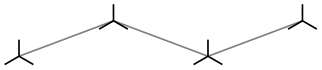
/pgfplots/every axis plot post(style, initially empty) 
The every axis plot post style can be used to overwrite parts (or all) of the drawing styles which are assigned for plots.
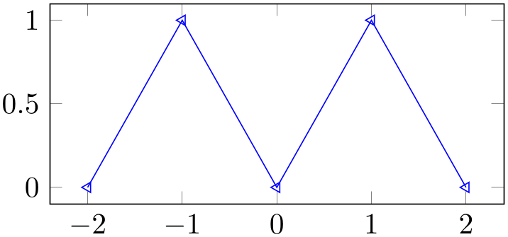
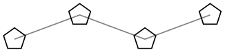
% Preamble: \pgfplotsset{width=7cm,compat=1.18}
% Overwrite any cycle list:
\pgfplotsset{
every axis plot post/.append style={
mark=triangle,
every mark/.append style={rotate=90},
},
}
\begin{tikzpicture}
\begin{axis}[y=2cm]
                \addplot coordinates
                {
(-2,0) (-1,1) (0,0) (1,1) (2,0)
};
\end{axis}
\end{tikzpicture}
Markers paths are not subjected to clipping as other parts of the figure. Markers are either drawn completely or not at all.
TikZ offers more options for marker fine tuning, please refer tothe PGF/TikZ manual for details.
4.7.2Line Styles
The following line styles are predefined in TikZ.
-
/tikz/solid(style, no value) 

-
/tikz/dotted(style, no value) 

-
/tikz/densely dotted(style, no value) 

-
/tikz/loosely dotted(style, no value) 

-
/tikz/dashed(style, no value) 

-
/tikz/densely dashed(style, no value) 

-
/tikz/loosely dashed(style, no value) 

-
/tikz/dashdotted(style, no value) 

-
/tikz/densely dashdotted(style, no value) 

-
/tikz/loosely dashdotted(style, no value) 

-
/tikz/dashdotdotted(style, no value) 

-
/tikz/densely dashdotdotted(style, no value) 

-
/tikz/loosely dashdotdotted(style, no value) 

since these styles apply to markers as well, you may want to consider using
in marker styles.
Besides linestyles, pgf also offers (a lot of) arrow heads. Please refer tothe PGF/TikZ manual for details.
4.7.3Edges and Their Parameters
When pgfplots connects points, it relies on pgf drawing parameters to create proper edges (and it only changes them in the every patch style).
It might occasionally be necessary to change these parameters:
-
/tikz/line cap=round|rect|butt (initially butt) 
-
/tikz/line join=round|bevel|miter (initially miter) 
-
/tikz/miter limit=
factor (initially 10)
These keys control how lines are joined at edges. Their description is beyond the scope of this manual, so interested readers should consultthe PGF/TikZ manual.
Here is just an example illustrating why it might be of interest to study these parameters:
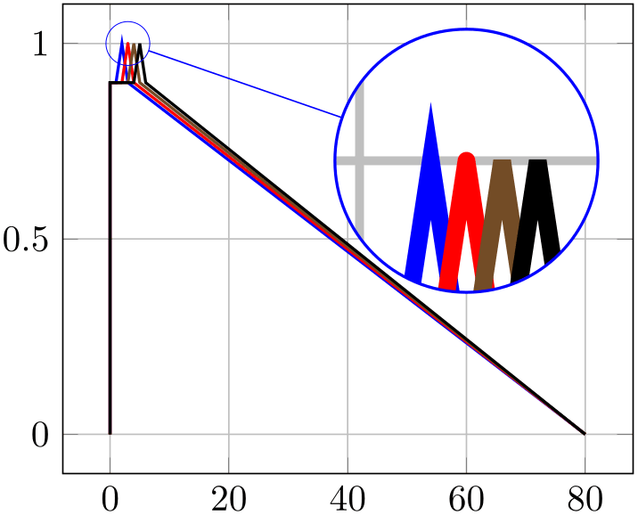
% Preamble: \pgfplotsset{width=7cm,compat=1.18}
% requires \usetikzlibrary{spy}
\begin{tikzpicture}[spy using outlines=
{circle, magnification=6, connect spies}]
\begin{axis}[no markers,grid=major,
every axis plot post/.append style={thick}]
\addplot coordinates
{(0, 0) (0, 0.9) (1, 0.9) (2, 1) (3, 0.9) (80, 0)};
\addplot+ [line join=round] coordinates
{(0, 0) (0, 0.9) (2, 0.9) (3, 1) (4, 0.9) (80, 0)};
\addplot+ [line join=bevel] coordinates
{(0, 0) (0, 0.9) (3, 0.9) (4, 1) (5, 0.9) (80, 0)};
\addplot+ [miter limit=5] coordinates
{(0, 0) (0, 0.9) (4, 0.9) (5, 1) (6, 0.9) (80, 0)};
\coordinate (spypoint) at (3,1);
\coordinate (magnifyglass) at (60,0.7);
\end{axis}
\spy [blue, size=2.5cm] on (spypoint)
in node[fill=white] at (magnifyglass);
\end{tikzpicture}
4.7.4Font Size and Line Width
Often, one wants to change line width and font sizes for plots. This can be done using the following options of TikZ.
-
/tikz/font={
font name} (initially \normalfont)
Sets the font which is to be used for text in nodes (like tick labels, legends or descriptions).
A font can be any LaTeX argument like \footnotesize or \small\bfseries.35
It may be useful to change fonts only for specific axis descriptions, for example using
\pgfplotsset{
tick label style={font=\small},
label style={font=\small},
legend style={font=\footnotesize},
}
See also the predefined styles normalsize, small and footnotesize in Section 4.10.2.
-
/tikz/line width={
dimension} (initially 0.4pt)
Sets the line width. Please note that line widths for tick lines and grid lines are predefined, so it may be necessary to override the styles every tick and every axis grid.
The line width key is changed quite often in TikZ. You should use
or
to change the overall line width. To also adjust ticks and grid lines, one can use
or styles like
The ‘every axis plot’ style can be used to change line widths for plots only.
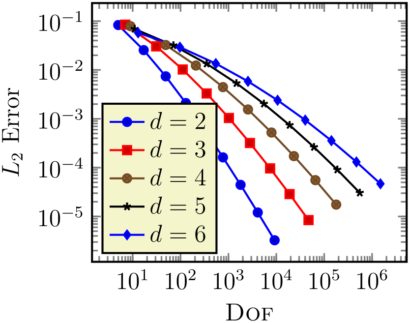
% Preamble: \pgfplotsset{width=7cm,compat=1.18}
\pgfplotsset{every axis/.append style={
font=\large,
line width=1pt,
tick style={line width=0.8pt}}}
\begin{tikzpicture}
\begin{loglogaxis}[
legend pos=south west,
xlabel=\textsc{Dof},
ylabel=$L_2$ Error
]
\addplot coordinates
{
(5,8.312e-02) (17,2.547e-02) (49,7.407e-03)
(129,2.102e-03) (321,5.874e-04) (769,1.623e-04)
(1793,4.442e-05) (4097,1.207e-05) (9217,3.261e-06)
};
\addplot coordinates{
(7,8.472e-02) (31,3.044e-02) (111,1.022e-02)
(351,3.303e-03) (1023,1.039e-03) (2815,3.196e-04)
(7423,9.658e-05) (18943,2.873e-05)
(47103,8.437e-06)};
\addplot coordinates{
(9,7.881e-02) (49,3.243e-02) (209,1.232e-02)
(769,4.454e-03) (2561,1.551e-03)
(7937,5.236e-04) (23297,1.723e-04)
(65537,5.545e-05) (178177,1.751e-05)};
\addplot coordinates{
(11,6.887e-02) (71,3.177e-02) (351,1.341e-02)
(1471,5.334e-03) (5503,2.027e-03)
(18943,7.415e-04) (61183,2.628e-04)
(187903,9.063e-05) (553983,3.053e-05)};
\addplot coordinates{
(13,5.755e-02) (97,2.925e-02) (545,1.351e-02)
(2561,5.842e-03) (10625,2.397e-03)
(40193,9.414e-04) (141569,3.564e-04)
(471041,1.308e-04) (1496065,4.670e-05)};
\legend{$d=2$,$d=3$,$d=4$,$d=5$,$d=6$}
\end{loglogaxis}
\end{tikzpicture}
The preceding example defines data which is used a couple of times throughout this manual; it is referenced by \plotcoords.
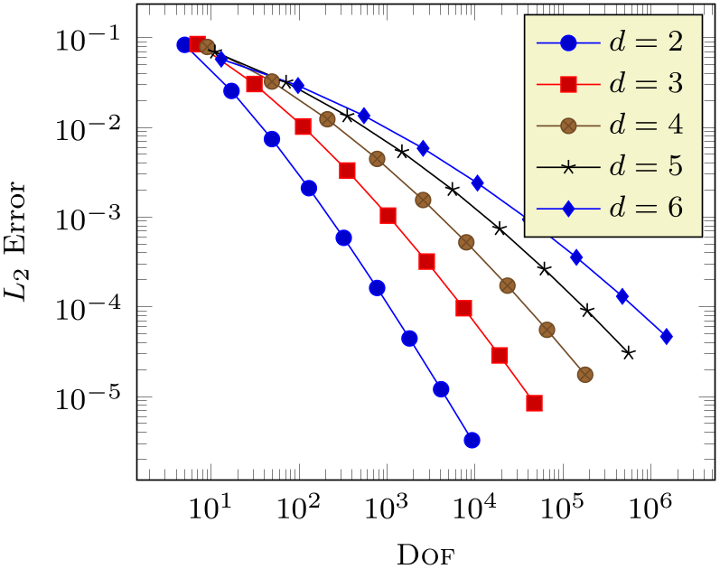
% Preamble: \pgfplotsset{width=7cm,compat=1.18}
\pgfplotsset{every axis/.append style={
font=\footnotesize,
thin,
tick style={ultra thin}},
}
\begin{tikzpicture}
\begin{loglogaxis}[
xlabel=\textsc{Dof},
ylabel=$L_2$ Error
]
% see above for this macro:
\plotcoords
\legend{$d=2$,$d=3$,$d=4$,$d=5$,$d=6$}
\end{loglogaxis}
\end{tikzpicture}
4.7.5Colors
pgf uses the color support of xcolor. Therefore, the main reference for how to specify colors is the xcolor manual [3]. The PGF/TikZ manual is the reference for how to select colors for specific purposes like drawing, filling, shading, patterns etc. This section contains a short overview over the specification of colors in [3] (which is not limited to pgfplots).
The package xcolor defines a set of predefined colors, namely
 red,
red,
 green,
 blue,
blue,
 cyan,
cyan,
 magenta,
 yellow,
 black,
 gray,
gray,
 white,
 darkgray,
 lightgray,
 brown,
 lime,
lime,
 olive,
 orange,
 pink,
pink,
 purple,
 teal,
teal,
 violet.
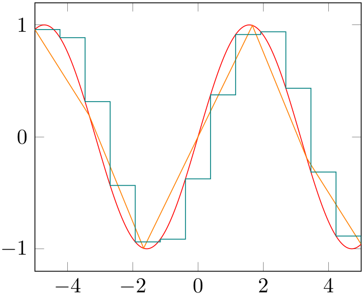
% Preamble: \pgfplotsset{width=7cm,compat=1.18}
\begin{tikzpicture}
\begin{axis}[enlarge x limits=false]
\addplot [red,samples=500] {sin(deg(x))};
\addplot [orange,samples=7] {sin(deg(x))};
\addplot [teal,const plot,samples=14]
{sin(deg(x))};
\end{axis}
\end{tikzpicture}
Besides predefined colors, it is possible to mix two (or more) colors. For example,
 red!30!white contains \(30\%\) of
 red and \(70\%\) of
 white. Consequently, one can build
 red!70!white to get \(70\%\) red and \(30\%\) white or
 red!10!white for \(10\%\) red and \(90\%\) white. This mixing can be done with
any color, for example
red!10!white for \(10\%\) red and \(90\%\) white. This mixing can be done with
any color, for example
 red!50!green,
 blue!50!yellow or
 green!60!black.
A different type of color mixing is supported, which allows to take \(100\%\) of each component. For example,
 rgb,2:red,1;green,1 will add \(1/2\) part
 red and \(1/2\) part
 green and we reproduced the example from above. Using the denominator \(1\) instead of \(2\) leads
to
green and we reproduced the example from above. Using the denominator \(1\) instead of \(2\) leads
to
 rgb,1:red,1;green,1 which uses \(1\) part
 red and \(1\) part
 green. Many programs allow to select pieces between \(0,\dotsc ,255\), so a denominator of \(255\) is useful.
Consequently,
green. Many programs allow to select pieces between \(0,\dotsc ,255\), so a denominator of \(255\) is useful.
Consequently,
 rgb,255:red,231;green,84;blue,121 uses \(231/255\) red,
\(84/255\) green and \(121/255\). This corresponds to the standard RGB color \((231,84,121)\). Other examples are
rgb,255:red,231;green,84;blue,121 uses \(231/255\) red,
\(84/255\) green and \(121/255\). This corresponds to the standard RGB color \((231,84,121)\). Other examples are
 rgb,255:red,32;green,127;blue,43,
 rgb,255:red,178;green,127;blue,43,
 rgb,255:red,169;green,178;blue,43.
It is also possible to use RGB values, the HSV color model, the CMY (or CMYK) models, or the HTML color syntax directly. However, this requires some more programming. I suppose this is the fastest (and probably the most uncomfortable) method to use colors. For example,

creates the color with \(100\%\)
 red, \(100\%\)
 green and \(0\%\)
 blue;
blue;

creates the color with \(60\%\)
 cyan, \(90\%\)
 magenta, \(50\%\)
 yellow and \(10\%\)
 black;

creates the color with \(208/255\) pieces red, \(178/255\) pieces green and \(43\) pieces blue, specified in standard HTML notation. Please refer to the xcolor manual [3] for more details and color models.
The xcolor package provides even more methods to combine colors, among them the prefix ‘-’
(minus) which changes the color into its complementary color ( -black,
 -white,
 -red) or color wheel calculations. Please refer to the
xcolor manual [3].
-red) or color wheel calculations. Please refer to the
xcolor manual [3].
-
/tikz/color={
a color}
-
/tikz/draw={
stroke color}
-
/tikz/fill={
fill color}
These keys are (generally) used to set
colors. Use color to set the color for both drawing and filling.
Instead of color={color name} you can simply write
color name. The draw and
fill keys only set colors for stroking and filling, respectively.
Use draw=none to disable drawing and fill=none to disable filling.36
Since these keys belong to TikZ, the complete documentation can be found in the PGF/TikZ manual, Section “Specifying a Color”.
36 Up to now, plot marks always have a stroke color (some also have a fill color). This restriction may be lifted in upcoming versions.
4.7.5.1Color Spaces
Since pgfplots relies on xcolor, all mechanisms of xcolor to define color spaces apply here as well.
One of the most useful approaches is global color space conversion: if you want a document which contains only colors in the cmyk color spaces, you can say
\usepackage[cmyk]{xcolor}
\usepackage{pgfplots}
in order to convert all colors of the entire document (including all shaded) to cmyk.
The same can be achieved by means of the xcolor statement \selectcolormodel.
4.7.6Color Maps
A “color map” is a sequence of colors with smooth transitions between them. Color maps are often used to visualize “color data” in plots: in this case, a plot has the position coordinates \((x,y)\) and some additional scalar value (point meta) which can be used as “color data”. The smallest encountered point meta is then mapped to the first color of a colormap, the largest encountered value of point meta is mapped to the last color of a colormap, and interpolation happens in-between.
-
/pgfplots/colormap name={
color map name} (initially hot)
Changes the current color map to the already defined map
named
color map name. The predefined color maps are
| viridis | |
| hot |
The definition can be found in the documentation for colormap/hot and colormap/viridis, respectively. These, and further color maps, are described below.
Color maps can be used, for example, in scatter plots and surface plots.
You can use colormap to create new color maps (see below).
-
/pgfplots/colormap={
name}{color specification}
Defines a new colormap named
name
according to
color specification
and activates it using colormap name={name}.
A simple
color specification
is just a sequence of color definitions of type
color type=(color value)
separated by either white spaces or semicolon or comma:
\pgfplotsset{colormap={CM}{rgb=(0,0,1) color=(black) rgb255=(238,140,238)}}
Here, the three input colors form the left end, middle point, and right end of the interval, respectively. A couple of
color types are available, the
color value
depends on the actual
color type
which is shown below in all detail. Most
colormap definitions use the simple form and merely list
suitable color definitions.
A more advanced
color specification
is one which defines both colors and positions in order to define the place of each color. In this case,
pgfplots offers the syntax
color type(offset)=(color value):
\pgfplotsset{colormap={CM}{rgb(-500)=(0,0,1) color(0)=(black) rgb255(1500)=(238,140,238)}}
This syntax allows to distribute colors over the interval using nonuniform distances.
pgfplots up to and including version \(1.13\) offered just rudimentary support for nonuniform color maps. You need to write compat=1.14 or higher in order to make use of nonuniform color maps.
The positions can be arbitrary numbers (or dimensions),37 but each new color must come with a larger position than its preceding one. The position can be omitted in which case it will be deduced from the context: if the first two colors have no position, the first will receive position \(0\) and the second will receive position “\(1\text {cm}\)”. All following ones receive the last encountered mesh width. Note that nonuniform positions make a real difference in conjunction with colormap access=piecewise const.
The precise input format is described in the following section.
4.7.6.1Colormap Input Format Reference
Each entry in
color specification
has the form
color model(position)=(arguments) or
special mode(position)=(argument of colormap name)
where the most common form is to specify a color using a
color model
like rgb=(0,0.5,1). The
special modes are discussed later in Section 4.7.6.4 on
page (page for section 4.7.6.4); they
are useful to access colors of existing colormaps. The
position
argument is optional and defaults to \(0\) for the first color, \(1\text {cm}\) for the second, and an automatically deduced
mesh grid for all following ones. The number range of
position
is arbitrary. Note that pgfplots merely remembers the relative distances of the
positions, not their absolute values. Consequently, a color map with positions \(0,1,2\) is equivalent to one with \(0,10,20\) or
\(-10,0,10\) or \(-1100,-1000,-900\). pgfplots maps the input positions to the range \([0,1000]\)
internally and works with these numbers. Each new color must have a
position
which is larger than the preceding one.
Available choices for
color model
are
-
rgb which expects
arguments
of the form (red,green,blue) where each component is in the interval \([0,1]\),
-
rgb255 which is similar to rgb except that each component is expected in the interval [0,255],
-
gray in which case
arguments
is a single number in the interval \([0,1]\),
-
color in which case
arguments
contains a predefined (named) color like ‘red’ or a color expression like ‘red!50’,
-
cmyk which expects
arguments
of the form (cyan,magenta,yellow,black) where each component is in the interval \([0,1]\),
-
cmyk255 which is the same as cmyk but expects components in the interval \([0,255]\),
-
cmy which expects
arguments
of the form (cyan,magenta,yellow) where each component is in the interval \([0,1]\),
-
hsb which expects
arguments
of the form (hue,saturation,brightness) where each component is in the interval \([0,1]\),
-
Hsb which is the same as hsb except that
hue
is accepted in the interval \([0,360]\) (degree),
-
HTML which is similar to rgb255 except that each component is expected to be a hex number between 00 and FF,
-
wave which expects a single wave length as numeric argument in the range \([363,814]\).
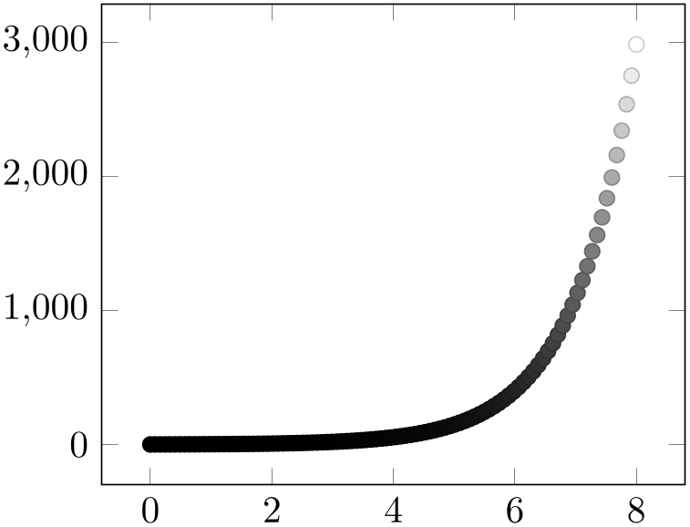
% Preamble: \pgfplotsset{width=7cm,compat=1.18}
\begin{tikzpicture}
\begin{axis}[
colormap={bw}{
gray(0cm)=(0);
gray(1cm)=(1);
},
]
\addplot+ [
scatter,
only marks,
domain=0:8,
samples=100,
] {exp(x)};
\end{axis}
\end{tikzpicture}
The choice of
positions
influences the processing time: a uniform distance between the
positions
allows more efficient lookup than nonuniform distances. If there is no visual difference and it does not hurt with respect to
the number of data points, prefer color maps with uniform distances over nonuniform maps. Note that nonuniform maps make a
huge difference in conjunction with
colormap access=piecewise constant.
pgfplots provides a simple way to map a nonuniform color definition to a uniform one: write the
target mesh width as first item in the specification. pgfplots will perform this
interpolation automatically, provided all encountered
positions
can be mapped to the target grid:
% non-uniform spacing example: the mesh width is provided as first
% part of the specification.
\pgfplotsset{colormap={violetnew}
{[1cm] rgb255(0cm)=(25,25,122) color(1cm)=(white) rgb255(5cm)=(238,140,238)}}
In this last example, the mesh width has been provided explicitly and pgfplots interpolates the missing grid points on its own. It is an error if the provided positions are no multiple of the mesh width.
4.7.6.2The Colorspace of a Colormap
Attention: this section is essentially superfluous if you have configured the xcolor package to override color spaces globally (for example by means of \usepackage[cmyk]{xcolor} before loading pgfplots), see the end of this subsection.
Even though a colormap accepts lots of color spaces on input (in fact, it accepts most or all that xcolor provides), the output color of a colorspace has strict limitations. The output colorspace is the one in which pgfplots interpolates between two other colors. To this end, it transforms input colors to the output color space. The output colorspace is also referred to as “the colorspace of a colormap”.
There are three supported color spaces for a colormap: the GRAY, RGB, and CMYK color spaces. Each access into a colormap requires linear interpolation which is performed in its color space. Color spaces make a difference: colors in different color spaces may be represented differently, depending on the output device. Many printers use CMYK for color printing, so providing CMYK colors might improve the printing quality on a color printer. The RGB color space is often used for display devices. The predefined colormaps in pgfplots all use RGB.
Whenever a new colormap is created, pgfplots determines an associated color space. Then, each color in this specific colormap will be represented in its associated color space (converting colors automatically if necessary). Furthermore, every access into the colormap will be performed in its associated color space and every returned mapped color will be represented with respect to this color space. Furthermore, every shading generated by shader=interp will be represented with respect to the colormap’s associated color space.
The color space is chosen as follows: in case
colormap default colorspace=auto
(the initial configuration), the color space depends on the first encountered color in
color specification. For rgb or gray or
color, the associated color space will be RGB (as it was in all earlier versions of pgfplots). For
cmyk, the associated color space will be CMYK. If
colormap default colorspace is either
gray, rgb or cmyk, this specific color space is used and every color is converted automatically.
-
/pgfplots/colormap default colorspace=auto|gray|rgb|cmyk (initially auto) 
Allows to set the color space of every newly created colormap. The choices are explained in the previous paragraph.
It is impossible to change the color space of an existing colormap; recreate it if conversion is required.
The macro \pgfplotscolormapgetcolorspace{name} defines \pgfplotsretval to contain the color space of an existing
colormap name, if you are in doubt.
Note that this option has no effect if you told xcolor to override the color space globally. More precisely, the use of
\usepackage[cmyk]{xcolor}
or, alternatively,
will cause all colors to be converted to cmyk, and pgfplots honors this configuration. Consequently, both these statements cause all colors to be interpolated in the desired color space, and all output colors will use this colorspace. This is typically exactly what you need.
4.7.6.3Predefined Colormaps
Available color maps are shown below.
-
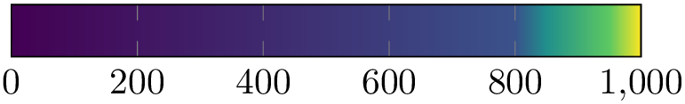
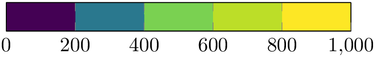
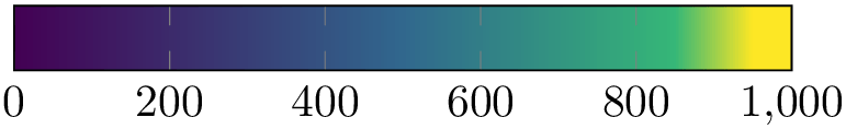
/pgfplots/colormap/viridis(style, no value) 
-
• its color distribution is perceptually uniform (compare the definition in the link below),
-
• it is suitable for moderate forms of color blindness,
-
• it is still good when printed in black and white.
A style which installs the colormap “viridis” which has been defined by Stèfan van der Walt and Nathaniel Smith for Matplotlib. It is designated to be the default colormap for Matplotlib starting with version 2.0 and is released under the CC038.
The choice viridis is a downsampled copy included in pgfplots.
This colormap has considerably better properties compared to other choices:
Details about these properties can be found in http://bids.github.io/colormap.
Please use the choice colormap name=viridis as this makes uses of the predefined colormap whereas colormap/viridis will redefine it.
There is also a high resolution copy of viridis which is called colormap/viridis high res in the colormaps library. It resembles the original resolution of the authors, but it is visually almost identically to viridis and requires less resources in TeX.
-
/pgfplots/colormap/hot2(style, no value) 
A style which is equivalent to
\pgfplotsset{
/pgfplots/colormap={hot2}{[1cm]rgb255(0cm)=(0,0,0) rgb255(3cm)=(255,0,0)
rgb255(6cm)=(255,255,0) rgb255(8cm)=(255,255,255)}
}
Note that this particular choice ships directly with pgfplots, you do not need to load the colormaps library for this value.
This colormap is similar to one shipped with Matlab® under a similar name.
-
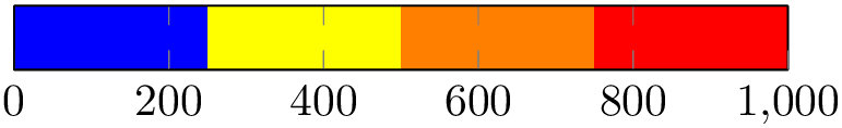
/pgfplots/colormap/jet(style, no value) 
A style which is equivalent to
\pgfplotsset{
/pgfplots/colormap={jet}{rgb255(0cm)=(0,0,128) rgb255(1cm)=(0,0,255)
rgb255(3cm)=(0,255,255) rgb255(5cm)=(255,255,0) rgb255(7cm)=(255,0,0) rgb255(8cm)=(128,0,0)}
}
This colormap is similar to one shipped with Matlab® under a similar name.
-
/pgfplots/colormap/blackwhite(style, no value) 
A style which is equivalent to
-
/pgfplots/colormap/bluered(style, no value) 
A style which is equivalent to
\pgfplotsset{
colormap={bluered}{
                            rgb255(0cm)=(0,0,180); rgb255(1cm)=(0,255,255);
                    rgb255(2cm)=(100,255,0);
                            rgb255(3cm)=(255,255,0); rgb255(4cm)=(255,0,0);
                    rgb255(5cm)=(128,0,0)}
}
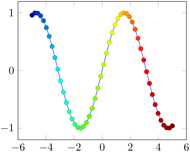
% Preamble: \pgfplotsset{width=7cm,compat=1.18}
\begin{tikzpicture}
\begin{axis}[colormap/bluered]
\addplot+ [scatter,
scatter src=x,samples=50]
{sin(deg(x))};
\end{axis}
\end{tikzpicture}
The style bluered (re)defines the color map and activates it. TeX will be slightly faster if you call \pgfplotsset{colormap/bluered} in the preamble (to create the color map once) and use colormap name=bluered whenever you need it. This remark holds for every color map style which follows. But you can simply ignore this remark.
-
/pgfplots/colormap/cool(style, no value) 
A style which is equivalent to
\pgfplotsset{
colormap={cool}{rgb255(0cm)=(255,255,255); rgb255(1cm)=(0,128,255); rgb255(2cm)=(255,0,255)}
}
-
/pgfplots/colormap/greenyellow(style, no value) 
A style which is equivalent to
-
/pgfplots/colormap/redyellow(style, no value) 
A style which is equivalent to
-
/pgfplots/colormap/violet(style, no value) 
A style which is equivalent to
-
\pgfplotscolormaptoshadingspec{
colormap name}{right end size}{\macro}
A command which converts a colormap into a pgf shading’s color specification. It can be used in commands like \pgfdeclare...shading (see the PGF/TikZ manual for details).
The first argument is the name of a (defined) colormap, the second the rightmost dimension of the specification. The result
will be stored in
\macro.
% convert `hot' -> \result
\pgfplotscolormaptoshadingspec{hot}{8cm}\result
% define and use a shading in pgf:
\def\tempb{\pgfdeclarehorizontalshading{tempshading}{1cm}}%
% where `\result' is inserted as last argument:
\expandafter\tempb\expandafter{\result}%
\pgfuseshading{tempshading}%
The usage of the result
\macro
is a little bit low-level.
pgf shadings are always represented with respect to the RGB color space. Consequently, even CMYK
colormap names will result in an RGB shading specification when using this method.39
-
\pgfplotscolorbardrawstandalone[
options]
A command which draws a tikzpicture and a colorbar using the current colorbar settings inside of it. Its purpose is to simplify the documentation.
Since this colorbar is a “standalone” picture, it defines the following options
before it evaluates
options
and draws the colorbar.
-
\pgfplotscolormaptodatafile[
options]{colormap name}{output file}
-
/pgfplots//pgfplots/colormap/output each nth=
num (initially 1)
-
/pgfplots//pgfplots/colormap/output format=cvs|native (initially csv) 
Allows to export colormap data to a file.
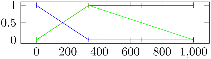
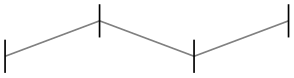
% Preamble: \pgfplotsset{width=7cm,compat=1.18}
\begin{tikzpicture}
\begin{axis}[y=1cm,table/col sep=comma]
\pgfplotscolormaptodatafile{hot}{hot.dat}
\addplot[red,mark=|] table[y index=1] {hot.dat};
\addplot[green,mark=|] table[y index=2] {hot.dat};
\addplot[blue,mark=|] table[y index=3] {hot.dat};
\end{axis}
\end{tikzpicture}
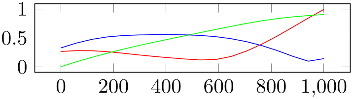
% Preamble: \pgfplotsset{width=7cm,compat=1.18}
\begin{tikzpicture}
\begin{axis}[y=1cm,table/col sep=comma]
\pgfplotscolormaptodatafile{viridis}{viridis.dat}
\addplot[red] table[y index=1] {viridis.dat};
\addplot[green] table[y index=2] {viridis.dat};
\addplot[blue] table[y index=3] {viridis.dat};
\end{axis}
\end{tikzpicture}
Valid
options
are
Allows
to downsample the color map by writing only each
num’s entry.
The choice csv generates a CSV file where the first column is the offset of the color map and all following are the color components.
The choice native generates a TeX file which can be \input in order to define the colormap for use in pgfplots.
Note that there are more available choices of colormaps in the associated libraries, name in the colorbrewer library and in the colormaps library which need to be loaded by means of \usepgfplotslibrary{colorbrewer,colormaps}.
38 https://creativecommons.org/about/cc0
39 In case pgf should someday support CMYK shadings and you still see this remark, you can add the macro definition \def\pgfplotscolormaptoshadingspectorgb{0} to your preamble.
4.7.6.4Building Colormaps based on other Colormaps
A colormap definition of sorts colormap={name}{color specification} typically consists of
color specifications
made up from single colors, each with its own
color model. As outlined in Section 4.7.6.1, each entry in
color specification
has the form
color model(position)=(arguments) or
special mode(position)=(argument of colormap name).
This section explains how to make use of
special mode
in order to build colormaps based on existing colormaps. To this end, pgfplots offers the following values inside of a
color specification:
-
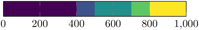
1. samples of colormap(
position)=(number of colormap name) or
samples of colormap(position)=(number) or
samples of colormap(position)={number of colormap name, options}
This method takes a
colormap name
on input, samples
number
colors from it (using a uniform mesh width) and inserts it into the currently built
colormap. It is equivalent to the choice colors of colormap(position)=(0,h,...,1000) with h chosen such that you get
number
samples positioned at an equidistant grid.
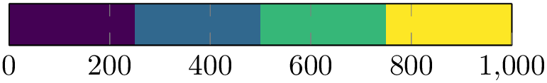
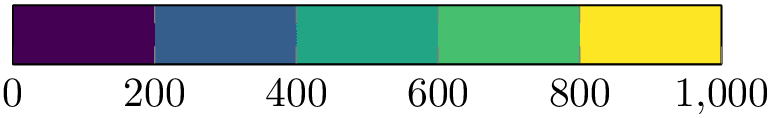
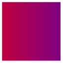
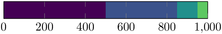
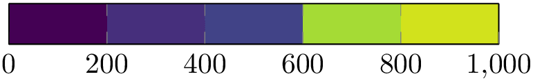
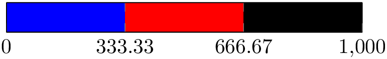
\pgfplotscolorbardrawstandalone[colormap={example}{samples of colormap=(4 of viridis)},colorbar horizontal,colormap access=const,]
\pgfplotscolorbardrawstandalone[colormap={example}{samples of colormap=(4 of viridis)},colorbar horizontal,colormap access=map,]The special suffix “ of
colormap name” is optional; it defaults to the current value of
colormap name:
\pgfplotscolorbardrawstandalone[colormap={example}{samples of colormap=(4)},colorbar horizontal,colormap access=const,]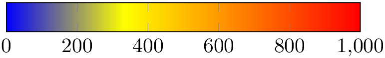
\pgfplotscolorbardrawstandalone[colormap={example}{samples of colormap=(4)},colorbar horizontal,colormap access=map,]The argument can be surrounded by round braces or curly braces, both is accepted. pgfplots also accepts a sequence of options inside of the argument and curly braces are best applied if options are needed:
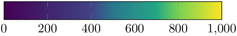
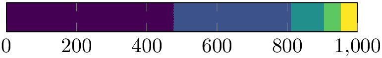
\pgfplotscolorbardrawstandalone[colormap={example}{samples of colormap={5 of viridis,target pos={0,800,850,950,1000},}},colorbar horizontal,colormap access=map,]
\pgfplotscolorbardrawstandalone[colormap={example}{% simpler alternative:% of colormap={viridis,target pos={...}}samples of colormap={5 of viridis,target pos={0,400,500,700,800,1000},sample for=const,}},colorbar horizontal,colormap access=const,]The use of options inside of the argument is discussed in the next subsection, see of colormap and target pos.
As with normal color definitions, the
position
argument is optional and can be omitted. If it is given, it is used for the first encountered item in the list, all others
are deduced automatically. If both
target pos and
position
are given,
position
is ignored.
Note that pgfplots offers a special syntax for target pos and a sampled colormap:
\pgfplotscolorbardrawstandalone[colormap={example}{of colormap={viridis,target pos={0,400,500,700,800,1000},sample for=const,}},colorbar horizontal,colormap access=const,]This syntax also samples colors from the source colormap (viridis here). It chooses enough samples to satisfy the given target pos; see the documentation for ‘of colormap’ for details.
-
2. index of colormap(
position)=(index of colormap name) or
index of colormap(position)=(index)
This key allows to identify a single color of
colormap name
and use it as part of
color specification. The
index
is a numeric index \(0,1,\dotsc ,N-1\) where \(N\) is the size of
colormap name.
\pgfplotscolorbardrawstandalone[colormap={example}{color=(green),index of colormap=(2 of viridis)},colorbar horizontal,colormap access=const,]Note that index of colormap is also available as key for drawing operations:
-
/pgfplots/index of colormap=
index
of
colormap name
Selects the specified color of
colormap name
using the special color name ‘.’, and assigns
color=.:

\pgfplotsset{colormap={example}{color=(red) color=(blue)}}\tikz \draw[index of colormap=0 of example] (0,0) -- (1,0);
\pgfplotsset{colormap={example}{color=(red) color=(blue)}}\tikz \fill[index of colormap=1 of example] (0,0) rectangle (1,1);Note that some drawing instructions require more than setting color. In this case, you have to reference the color ‘.’ after the key:
\pgfplotsset{colormap={example}{color=(red) color=(blue)}}\tikz \shade[index of colormap=0 of example,left color=.,color of colormap=500 of example,right color=.] (0,0) rectangle (1,1);All special remarks of samples of colormap (like curly braces, option list support, positions) apply here as well.
-
-
3. indices of colormap(
position)=(list of indices of colormap name) or
indices of colormap(position)=(list of indices)
A convenience key which is equivalent to a sequence of index of colormap(
position), one for each element in
list. The
list
is evaluated using \foreach. Note that you need round braces around the argument.
\pgfplotscolorbardrawstandalone[colormap={example}{indices of colormap=(0,5,10,12,\pgfplotscolormaplastindexof{viridis}of viridis)},colorbar horizontal,colormap access=const,]All special remarks of samples of colormap (like curly braces, option list support, positions) apply here as well.
-
4. color of colormap(
position)=(value of colormap name) or
color of colormap(position)=(value)
This key allows to interpolate a color within
colormap name
and use the result as part of
color specification. The interpolation point is a floating point number in the range \([0,1000]\) and is interpolated using
colormap access=map (i.e. using piecewise linear
interpolation).
Note that color of colormap is also available as key for drawing operations:
-
/pgfplots/color of colormap=
value
of
colormap name
Selects the specified color of
colormap name
using the special color name ‘.’, and assigns
color=.:
\pgfplotsset{colormap={example}{color=(red) color=(blue)}}\tikz \shade[color of colormap=250 of example,left color=.,color of colormap=500 of example,right color=.] (0,0) rectangle (1,1);All special remarks of samples of colormap (like curly braces, option list support, positions) apply here as well.
-
-
5. colors of colormap(
position)=(list of colormap name) or
colors of colormap(position)=(list) or
colors of colormap(position)={list of colormap name, options}
A convenience key which is equivalent to a sequence of color of colormap(
position), one for each element in
list. The
list
is evaluated using \foreach. Note that you need round braces around the argument.
\pgfplotscolorbardrawstandalone[colormap={example}{colors of colormap=(0,400,800,900,1000 of viridis)},colorbar horizontal,colormap access=const,]Note that colors of colormap is also available during cycle list definitions.
All special remarks of samples of colormap (like curly braces, option list support, positions) apply here as well.
-
6. of colormap(
position)=(colormap name, options)
Builds a new colormap by sampling enough colors from the input colormap name. This mode is one of two methods which samples colors from another colormap; it is to be preferred if you want to assign target pos. See also samples of colormap; it is simpler if you just want to specify a number of samples.
The syntax ‘of colormap=’ is most useful if you want to draw samples from another colormap at specific positions:
\pgfplotscolorbardrawstandalone[colormap={example}{of colormap={viridis,target pos={0,400,500,700,800,1000},},},colorbar horizontal,colormap access=map,]Here, pgfplots parses the
options. Each unidentified option is treated as either a value of ‘colormap name’ or as a style argument which defines a
colormap like
colormap/PuOr. The previous example identifies
colormap name=viridis (since viridis is
no known option) and assigns target pos. There are \(6\) samples which make up the colormap, these are drawn from viridis. Note that you do not need to
specify a
colormap name
in this context. If it is missing, the current value of
colormap name (i.e. the current colormap) will be
used.
Similarly, ‘of colormap’ can sample a colormap for use with colormap access=const:

\pgfplotscolorbardrawstandalone[colormap={example}{of colormap={viridis,target pos={0,400,500,700,800,1000},sample for=const,},},colorbar horizontal,colormap access=const]Note that you need to write sample for=const in this context such that pgfplots knows that the result is to be used in conjunction with colormap access=const. The details are specified below.
As with all colormap building blocks, the target pos can have an arbitrary number range. However, the absolute values are meaningless; they are always mapped to the range \([0,1000]\). Only their relative distances are of importance when it comes to the colormap as such:
\pgfplotscolorbardrawstandalone[colormap={example}{of colormap={viridis,target pos={-10,-3,0,1,2},sample for=const,},},colorbar horizontal,colormap access=const]However, if the point meta range equals the colormap definition range, you see that they fit exactly:
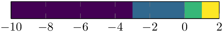
\pgfplotscolorbardrawstandalone[colormap={example}{of colormap={viridis,target pos={-10,-3,0,1,2},sample for=const,},},point meta min=-10,point meta max=2,colorbar horizontal,colormap access=const]Note that you can use xtick=data or ytick=data inside of the colorbar styles in order to place tick labels at the colormap’s positions:
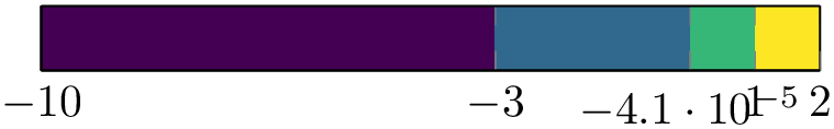
\pgfplotscolorbardrawstandalone[colormap={example}{of colormap={viridis,target pos={-10,-3,0,1,2},sample for=const,},},point meta min=-10,point meta max=2,colorbar horizontal,colorbar style={xtick=data},colormap access=const]Finally, ‘of colormap’ can be used to copy another colormap: if there are no suitable hints how to build a new colormap, pgfplots copies the input map:
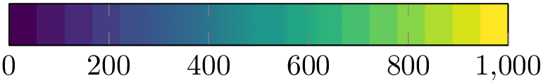
\pgfplotscolorbardrawstandalone[colormap={example}{of colormap={viridis},},colorbar horizontal,colormap access=const]The
options
are accepted by all colormap building blocks: you can also specify them after
samples of colormap or
colors of colormap if needed.
The following options are available:
-
/pgfplots/of colormap/target pos={
position(s)} (initially empty)
Allows to define the
position
for zero, one, or more of the involved colors. An empty value means to use the argument in round braces ‘(position)’ in the definition, for example the value \(100\) in color of colormap(100)=(4). This is
sufficient if there is just one color involved. However, if
target pos has a non-empty value, it
overrides the (position) argument.
The key target pos is primarily intended to provide positions for more than one color definition, in particular in the context of ‘of colormap’. In this context, as many
position(s)
as specified are used.
If you have colors of colormap and a non-empty value of target pos, pgfplots will use as many target positions as available. If there are too few to cover all involved colors, the remaining ones are deduced automatically. More precisely: pgfplots will use the current mesh width as distance to the previous position. The “current mesh width” is defined as the smallest difference between adjacent positions. Excess positions will be ignored (and a warning is written into the logfile).
Note that target pos requires attention when used together with colormap access=const: in this case, there are intervals with constant color and the positions become interval boundaries. Consequently, \(N\) elements in target pos make up \(N-1\) different colors!
Note that target pos as option to samples of colormap is also possible. However, you have to specify all required positions and it is an error if the number does not match. If you also combine this case with sample for=const, you need \(N+1\) positions for \(N\) samples.
-
/pgfplots/of colormap/sample for=default|const (initially default) 
-
• In general, a colormap can be used with any value of colormap access. If there are no positions in the
colormap definition
(neither in round braces nor in
target pos), this works out of the box without any special attention.
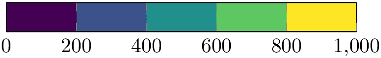
\pgfplotscolorbardrawstandalone[colormap={example}{samples of colormap={5 of viridis,},},colorbar horizontal,colormap access=const] -
• As soon as there are positions, pgfplots has a conflict if the colormap is used in the context of colormap access=const: it cannot enlarge the displayed limit, but it cannot respect both the given positions and the required number of colors! It has the choice to either omit one color, or to add an artificial position and rescale all other positions.
-
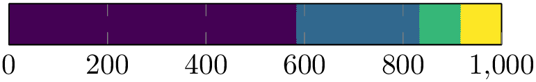
• The default strategy in pgfplots in the presence of colormap access=const and input positions is: pgfplots chooses to keep the input positions and omit one color.
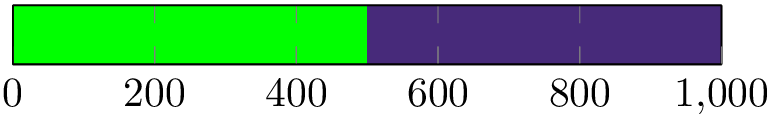
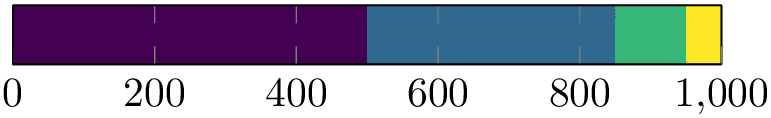
\pgfplotscolorbardrawstandalone[colormap={example}{of colormap={viridis,target pos={0,500,850,950,1000},},},colorbar horizontal,colormap access=const]Technically, this means that it implicitly sets colormap access/extra interval width=0 (the default is colormap access/extra interval width=h). The color associated with \(1000\) has no interval and is essentially invisible.
Restoring colormap access/extra interval width=h results in rescaled positions which is typically not what you want:
\pgfplotscolorbardrawstandalone[colormap={example}{samples of colormap={5 of viridis,target pos={0,500,850,950,1000},},},colormap access/extra interval width=h,colorbar horizontal,colormap access=const] -
• Finally, pgfplots offers sample for=const.
Applying sample for=const to ‘of colormap’ ensures that any given positions are respected. To this end, it reduces the number of available colors, but modifies the sampling procedure such that the entire input color range is visible in the result:
\pgfplotscolorbardrawstandalone[colormap={example}{of colormap={viridis,target pos={0,500,850,950,1000},sample for=const,},},colorbar horizontal,colormap access=const]Here, the result has \(4\) colors, but the rightmost color is also the rightmost color of the input map viridis. Note that of colormap has assigned an invisible color to the position \(1000\): this dummy color is defined to be the rightmost color of viridis. That means that if you define a colormap with sample for=const and use it with colormap access=map, the right end of the interval will be longer than expected:
\pgfplotscolorbardrawstandalone[colormap={example}{of colormap={viridis,target pos={0,500,850,950,1000},sample for=const,},},colorbar horizontal,colormap access=map]The strategy sample for=const applied to samples of colormap works in a similar way. Keep in mind that this combination requires to either omit target pos or to add exactly \(N+1\) target positions:
\pgfplotscolorbardrawstandalone[colormap={example}{samples of colormap={5 of viridis,target pos={0,100,500,850,950,1000},sample for=const,},},colorbar horizontal,colormap access=const]This results in correctly respected positions and a fully respected range of the input colormap.
This key allows to configure samples of colormap such that the resulting colormap is suitable for dedicated values of colormap access.
In particular, it allows to optimize
colormap definitions
which rely on sampling for the case
colormap access=const.
Note that the case colormap access\(\neq \)const typically requires no modification to this key and works best with the defaults.
The strategy colormap access=const means that colors are associated with entire intervals and no longer with single positions in the colormap. In this context, you have to write sample for=const such that pgfplots handles that correctly.
Here is the reference of colormaps and their significance with respect to sample for:
The key sample for applies whenever a
colormap definition
involves sampling (that means: only for of colormap and
samples of colormap). It does not apply for explicitly fixed colors. Its effect is that the number of samples is reduced by \(1\) and
the last provided sample is replicated once.
See also colormap access/extra interval width.
-
/pgfplots/of colormap/colormap access={
argument}
An alias for /pgfplots/colormap access={
argument}.
-
/pgfplots/of colormap/source range={
min:max} (initially 0:1000)
Defines the source range for interpolation-based specifications, i.e. for color of colormap and const color of colormap. It defaults to 0:1000 which means that only values in the interval \([0,1000]\) can be provided.
Changing the value allows to use any number range in order to identify numbers.
\pgfplotscolorbardrawstandalone[colormap={example}{colors of colormap={-30000,-10000,0,100000,110000 of viridis,source range=-30000:120000,},},colorbar horizontal,colormap access=const]Note that these building blocks can be combined as often as needed. This allows to combine different colormaps:
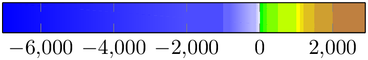
\pgfplotscolorbardrawstandalone[point meta min=-7046,point meta max=2895,colormap={whiteblue}{color=(blue) color=(white)},colormap={gb}{color=(green) color=(yellow)color=(brown)},colormap={CM}{of colormap={whiteblue,target pos={-7046,-6000,-5000,-3000,-1000,-750,-500,-250,-100,-50,0},sample for=const,},of colormap={gb,target pos={10,100,200,500,1000,1100,1200,1500,2000,2895},sample for=const,},},colorbar horizontal,colormap access=const]The previous example first defines the two simple colormaps whiteblue and gb. These are merely used as building blocks; they are not used for the visualization. Finally, the colormap CM consists of two of colormap specifications which resample the building blocks and assign specific target positions.
-
/pgfplots/of colormap/target pos min={
lower limit} (initially empty)
-
/pgfplots/of colormap/target pos min*={
lower limit} (initially empty)
-
/pgfplots/of colormap/target pos max={
upper limit} (initially empty)
-
/pgfplots/of colormap/target pos max*={
upper limit} (initially empty)
These keys allow to modify the argument of target pos. Their primary use is to simplify writing style definitions. Consequently, most users may want to ignore these keys and skip their documentation. The keys are unnecessary if the argument of target pos is used directly.
The versions without star (target pos min and target pos max) discard all elements of target pos which are outside of the bounds. The starred versions (target pos min* and target pos max*) also discard all which do not fit, but they ensure that the limit is part of target pos after the filtering.
These filtering limits come in handy if you want to select matching positions from a previously defined target pos, for example if the same target pos is part of a reusable style:

\pgfplotsset{of colormap/ocean height/.style={target pos={-12000,-10000,-6000,-5000,-3000,-1000,-750,-500,-250,-100,-50,0,10,100,200,500,1000,1100,1200,1500,2000,4000,6000,8000},},}\pgfplotscolorbardrawstandalone[point meta min=-7046,point meta max=2895,colormap={whiteblue}{color=(blue) color=(white)},colormap={gb}{color=(green) color=(yellow)color=(brown)},colormap={CM}{of colormap={whiteblue,ocean height,target pos min*=\pgfkeysvalueof{/pgfplots/point meta min},target pos max=0,sample for=const,},of colormap={gb,ocean height,target pos min=0.1,target pos max*=\pgfkeysvalueof{/pgfplots/point meta max},sample for=const,},},colorbar horizontal,colormap access=const]The example defines a style named ‘ocean height’ with a suitable list of positions somewhere in the document. Then, it defines a colormap ‘CM’ which makes use of these keys – but only in the range \([-7046,2895]\), and with a special combination of two other colormaps. The first of colormap specification selects only those target positions which fall in the range \([-7046,0]\) and ensures that \(-7046\) actually becomes an element of target pos. The second of colormap specification selects all in the range \([0.1,2895]\) and ensures that \(2895\) becomes an element of target pos. Note that the \(0.1\) merely serves as indicator to not select \(0\) again. Thus, the selection is essentially equivalent to
...target pos={-7046,-6000,-5000,-3000,-1000,-750,-500,-250,-100,-50,0}...target pos={10,100,200,500,1000,1100,1200,1500,2000,2895}with the exception that the predefined style defined a list of suitable positions. The colors taken from whiteblue are the same as if you would write samples of colormap={11}, i.e. they are drawn uniformly from the input colormap. Only their target position in the result is modified. The same applies to the colors taken from bg; they are drawn uniformly and moved to the prescribed boundaries.
pgfplots uses these keys in order to implement contour filled.
Note that a colormap definition is not bound to specific coordinates, although this makes a lot of sense in the context of contour plots. In principle, you can use the resulting colormap in any context, just as all other colormaps:
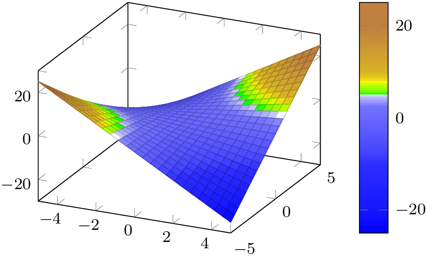
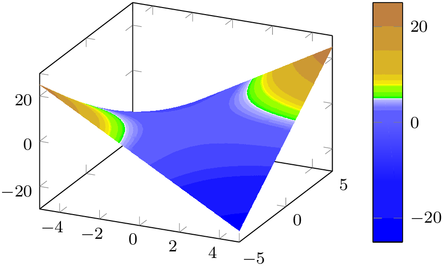
% Preamble: \pgfplotsset{width=7cm,compat=1.18}\pgfplotsset{colormap={whiteblue}{color=(blue) color=(white)},colormap={gb}{color=(green) color=(yellow)color=(brown)},of colormap/ocean height/.style={target pos={-12000,-10000,-6000,-5000,-3000,-1000,-750,-500,-250,-100,-50,0,10,100,200,500,1000,1100,1200,1500,2000,4000,6000,8000},},colormap={CM}{of colormap={whiteblue,ocean height,target pos max=0,sample for=const,},of colormap={gb,ocean height,target pos min=0.1,sample for=const,},},}\begin{tikzpicture}\begin{axis}[small,colorbar]\addplot3[surf] {x*y};\end{axis}\end{tikzpicture}~\begin{tikzpicture}\begin{axis}[small,colorbar,colorbar style={colormap access=const}]\addplot3[surf,shader=interp,colormap access=const] {x*y};\end{axis}\end{tikzpicture}Note that the last example has the same look as if it was produced by contour filled. The difference is that contour filled takes the input colormap and resamples it according to the selected contour levels. The example above is just a “normal” surface plot with a special colormap.
-
-
7. const color of colormap(
position)=(value of colormap name)
This key is almost the same as color of colormap mentioned above, but it uses the same functionality as colormap access=piecewise constant while it determines colors from the source color map (including colormap access/extra interval width). Note that the resulting colormap can still be used with any value of colormap access, including both colormap access=const and colormap access=map.
Note that const color of colormap is also available as key for drawing operations:
-
/pgfplots/const color of colormap=
value
of
colormap name
Selects the specified color of
colormap name
using the special color name ‘.’, and assigns
color=.:
\pgfplotsset{colormap={example}{color=(red) color=(blue) color=(yellow)}}\tikz \fill[const color of colormap=50 of example] (0,0) rectangle (1,1);\tikz \fill[const color of colormap=750 of example] (0,0) rectangle (1,1);All special remarks of samples of colormap (like curly braces, option list support, positions) apply here as well.
-
-
8. const colors of colormap(
position)=(list of colormap name)
A convenience key which is equivalent to a sequence of const color of colormap(
position), one for each element in
list. The
list
is evaluated using \foreach.
Note that const colors of colormap is also available during cycle list definitions.
All special remarks of samples of colormap (like curly braces, option list support, positions) apply here as well.
-
/pgfplots/colormap access/extra interval width={
fraction} (initially h)
this key is supposed to be a technical part of the implementation. You may want to skip its documentation as it typically works out of the box. You only need to respect sample for.
This key applies only to colormap access=piecewise constant: it ensures that each color in the colormap receives its own interval. This ensures that each color is actually visible in the output. Thus, each provided color resembles an interval. This is different from colormap access=map where each provided color resembles an interval boundary.
Normally, pgfplots, activates this feature if and only if it has automatically computed positions. Consequently, the following example implicitly uses extra interval width=h (the default):

\pgfplotscolorbardrawstandalone[
colormap={example}{
color=(blue)
color=(red)
color=(black)
},
colorbar horizontal,
colorbar style={xtick=data},
colormap access=const,
]
As soon as you provide positions manually, pgfplots defaults to extra interval width=0 in order to respect the input settings:
\pgfplotscolorbardrawstandalone[
colormap={example}{
color(0)=(blue)
color(500)=(red)
color(1000)=(black)
},
colorbar horizontal,
colorbar style={xtick=data},
colormap access=const,
]
Note that the positions make up the input nodes for the colormap with the consequence that the last color is unused; it merely serves as interval boundary. In this context, “provide manually” means positions in round braces or a non-empty value of target pos.
In order to override the input positions and get an extra interval, you have to set the option:
\pgfplotscolorbardrawstandalone[
colormap={example}{
color(0)=(blue)
color(500)=(red)
color(1000)=(black)
},
colorbar horizontal,
colorbar style={xtick=data},
colormap access/extra interval width=h,
colormap access=const,
]
Note how the extra interval of colormap access=const modifies the positions of the colormap definition: they are all shifted to the left and the chosen input positions are scaled accordingly. This becomes more apparent in the following example. First, we generate a colormap with the default settings which disables the extra interval, but omits the last (brightest) color:
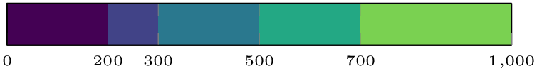
\pgfplotscolorbardrawstandalone[
colormap={nonuniform}{
of colormap={
viridis,
target pos={0,200,300,500,700,1000}
},
},
colorbar horizontal,
colormap access=const,
colorbar style={xtick=data,font=\tiny,
/pgf/number format/precision=0},
colormap access=const,
]
Next, we explicitly enable the extra interval and see that the input positions are scaled to the left. Note that they keep their relative distances, but the last color of the colormap is finally visible:
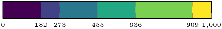
\pgfplotscolorbardrawstandalone[
colormap={nonuniform}{
of colormap={
viridis,
target pos={0,200,300,500,700,1000}
},
},
colorbar horizontal,
colormap access=const,
colormap access/extra interval width=h,
colorbar style={xtick=data,font=\tiny,
/pgf/number format/precision=0},
colormap access=const,
]
The last example relies on of colormap and a sampling procedure. In this context, pgfplots offers sample for=const which results in the expected look:
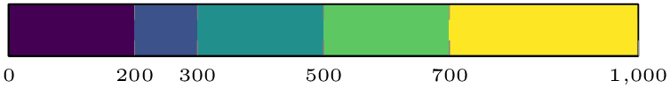
\pgfplotscolorbardrawstandalone[
colormap={nonuniform}{
of colormap={
viridis,
target pos={0,200,300,500,700,1000},
sample for=const,
},
},
colorbar horizontal,
colormap access=const,
colorbar style={xtick=data,font=\tiny,
/pgf/number format/precision=0},
colormap access=const,
]
Please refer to the documentation of sample for.
The default width of this interval is the mesh width of the color map (the value h), i.e. it will always be as large as the other intervals. If the color map has nonuniform distances, the smallest encountered mesh width is used for the extra interval. This can be seen if we omit the key and add some artificial color at the right end manually – we only need to ensure that the rightmost interval has the correct length. In our example above, the smallest mesh width is \(100\), so we can generate an equivalent result by means of

\pgfplotscolorbardrawstandalone[
colormap={nonuniform}{
of colormap={
viridis,
target pos={0,200,300,500,700,1000}
},
color(1100)=(red)
},
colorbar horizontal,
colormap access=const,
colorbar style={xtick=data,font=\tiny,
/pgf/number format/precision=0},
colormap access=const,
]
As already mentioned, colormap access=const ignores the rightmost color (“red”). Note that this approach is almost the same as the internal implementation of sample for=const.
The value of
colormap access/extra interval width=fraction
can also be used to customize the width of the artificial interval: it is a fraction of the total width and accepted values
are \(0\le \)fraction\(\le 0.9\) where \(0\) disables the extra interval and \(0.9\) corresponds to \(90\%\) of the resulting width. Any non-\(0\)
value for
fraction
creates an extra interval and its width is
fraction
percent of the entire color map. The special magic value
colormap access/extra interval width=h will use the colormap’s mesh width. If the colormap
has nonuniform distances, it will use the smallest encountered mesh width. This is the default.
Note that
fraction
is a property of the colormap. The key defines it for the current color map only. Defining a new
colormap uses the default width for the new
colormap (but keeps the configured value for the old
colormap).
at the time of this writing, uniform color maps only support the default interval width ‘h’ and
fraction\(=0\), further customization is only possible for nonuniform color maps. If you ever need to work around this limitation,
you should file a feature requests and move one of your color position until the colormap becomes a nonuniform colormap.
4.7.6.5Choosing a Colormap Entry as Normal Color
-
/pgfplots/color of colormap=
value
-
/pgfplots/color of colormap=
value
of
colormap name
[See also Section 4.7.6.4 on page (page for section 4.7.6.4) for how to employ this within colormap definitions]
Defines the TikZ color to be the
value
of
colormap name. If
colormap name
is omitted, the value of colormap name is evaluated
(i.e. the current colormap is used).
The argument
value
is expected to be a number in the range \([0,1000]\) where \(0\) resembles the lower end of the color map and \(1000\) the
upper end.
Current colormap (hot):

The key computes the requested color and calls color=.. Keep in mind
that the magic color name ‘.’ always reflects the “current color”, i.e. the result of
color=some color. Also keep in mind that color is a TikZ command which
merely defines the color, you also have to provide one of ‘draw’ or ‘fill’ such that it has an effect. Since ‘.’ is a normal color, we can write
draw=.!60!black to combine it with another color.
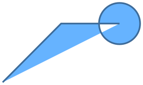
viridis:
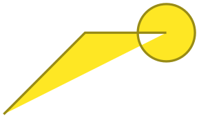
\pgfplotsset{colormap name=viridis}
\tikz\fill [color of colormap={1000},thick,
draw=.!60!black]
                            (0,0) --
                    (1,1) -- (2,1) circle (10pt);

The argument
colormap name
is either a valid argument of colormap name
or a style name like colormap/cool:
cool:
This last syntax allows to evaluate colormaps lazily. However, if you have many references to the same colormap, it makes sense to write \pgfplotsset{colormap/cool} first followed by many references to color of colormap={... of cool} in order to avoid unnecessary lazy evaluations.
It is possible to write lots of invocations without an explicit
colormap name, i.e. lots of invocations of sorts color of colormap=value. They will all use the colormap name which is
active at that time.
Note that there are actually keys with two key prefixes: /pgfplots/color of colormap and an alias /tikz/color of colormap. This allows to use the keys both for plain TikZ graphics and for pgfplots.
See also colormap access=map.
-
/pgfplots/index of colormap=
index
-
/pgfplots/index of colormap=
index
of
colormap name
-
\pgfplotscolormapsizeof{
colormap name}
-
\pgfplotscolormaplastindexof{
colormap name}
[See also Section 4.7.6.4 on page (page for section 4.7.6.4) for how to employ this within colormap definitions]
A variant of color of colormap which accesses the
colormap name
by index. Consequently, the argument
index
is an integer number in the range \(0,\dotsc ,N-1\) where \(N\) is the number of colors which define the
colormap name. A
index
outside of this range is automatically clipped to the upper bound.


\pgfplotsset{colormap/jet}
\foreach \i in {
0,...,\pgfplotscolormaplastindexof{jet}
}{
\tikz\fill [
index of colormap={\i of jet},
thick,
draw=.!60!black,
] (0,0) rectangle (10pt,6pt);
}
Expands to the number of colors which make up
colormap name.
If the argument
colormap name
is an unknown colormap, it expands to \(0\).
Expands to the last index of
colormap name, i.e. it is a convenience method to access \(N-1\).
If the argument
colormap name
is an unknown colormap, it expands to \(-1\).
See also colormap access=direct.
-
/pgfplots/const color of colormap=
value
-
/pgfplots/const color of colormap=
value
of
colormap name
[See also Section 4.7.6.4 on page (page for section 4.7.6.4) for how to employ this within colormap definitions]
Defines the TikZ color to be the
value
of
colormap name. If
colormap name
is omitted, the value of colormap name is evaluated
(i.e. the current colormap is used).
This key is almost the same as color of colormap, except that it uses colormap access=piecewise constant in order to determine the interpolated value.
4.7.7Cycle Lists – Options Controlling Line Styles
-
/pgfplots/cycle list={
list}
-
/pgfplots/cycle list name={
name} (initially color)
Allows to specify a list of plot specifications which
will be used for each \addplot command without explicit
plot specification. Thus, the currently active
cycle list will be used if you write either
\addplot+[keys] ...; or if you don’t use square brackets as in
\addplot[explicit plot specification] ...;.
The list element with index \(i\) will be chosen where \(i\) is the index of the current \addplot command (see also the cycle list shift key which allows to use \(i+n\) instead). This indexing does also include plot commands which don’t use the cycle list.
There are several possibilities to change the currently active cycle list:
4.7.7.1Predefined Lists
Use one of the predefined lists,40
-
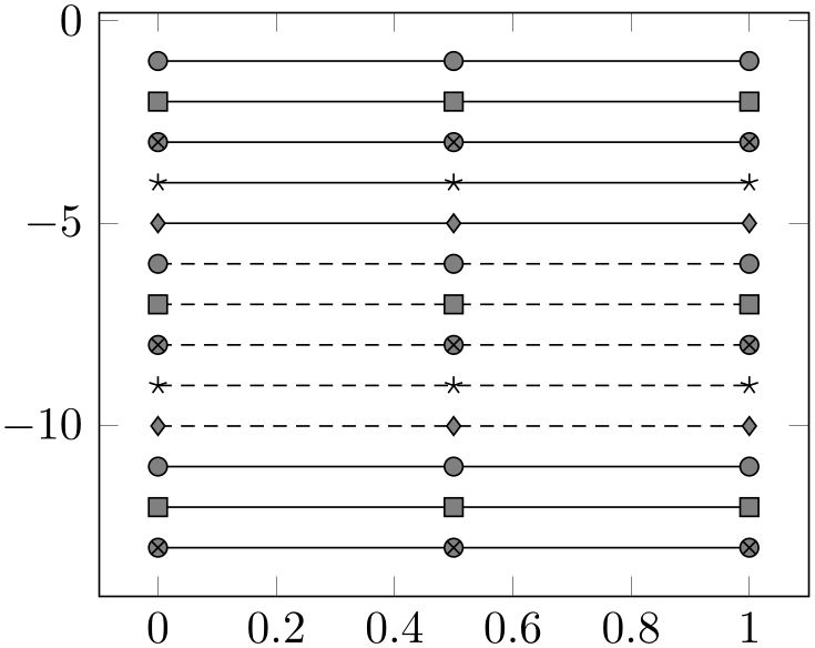
• color (from top to bottom)
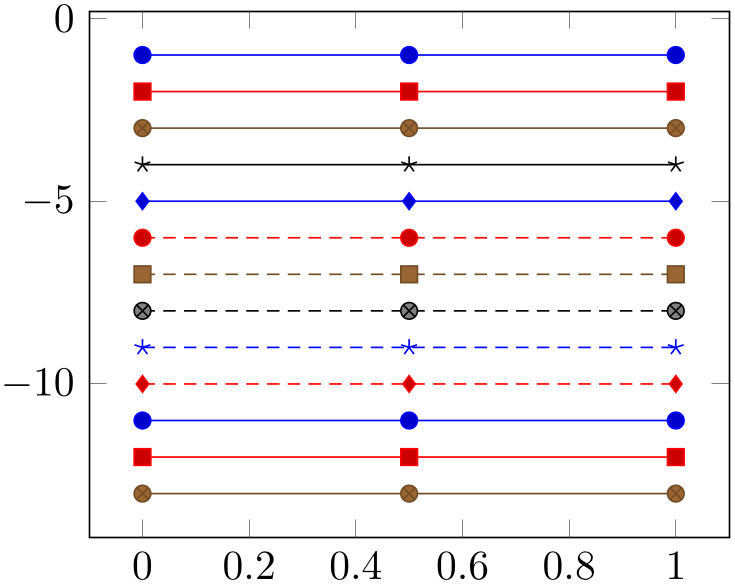
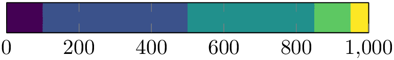
% Preamble: \pgfplotsset{width=7cm,compat=1.18}\begin{tikzpicture}\begin{axis}[stack plots=y,stack dir=minus,cycle list name=color,]\addplot coordinates {(0,1) (0.5,1) (1,1)};\addplot coordinates {(0,1) (0.5,1) (1,1)};\addplot coordinates {(0,1) (0.5,1) (1,1)};\addplot coordinates {(0,1) (0.5,1) (1,1)};\addplot coordinates {(0,1) (0.5,1) (1,1)};\addplot coordinates {(0,1) (0.5,1) (1,1)};\addplot coordinates {(0,1) (0.5,1) (1,1)};\addplot coordinates {(0,1) (0.5,1) (1,1)};\addplot coordinates {(0,1) (0.5,1) (1,1)};\addplot coordinates {(0,1) (0.5,1) (1,1)};\addplot coordinates {(0,1) (0.5,1) (1,1)};\addplot coordinates {(0,1) (0.5,1) (1,1)};\addplot coordinates {(0,1) (0.5,1) (1,1)};\end{axis}\end{tikzpicture} -
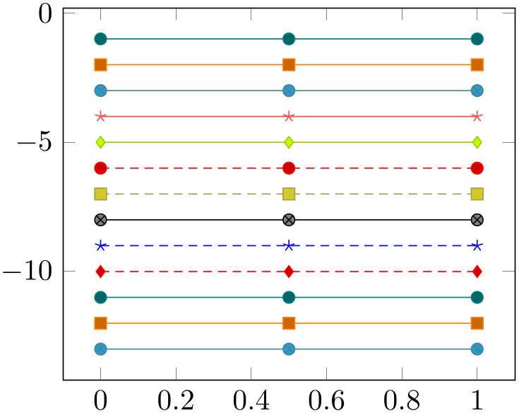
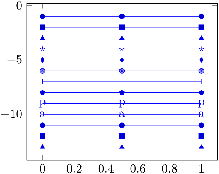
% Preamble: \pgfplotsset{width=7cm,compat=1.18}\begin{tikzpicture}\begin{axis}[stack plots=y,stack dir=minus,cycle list name=exotic,]\addplot coordinates {(0,1) (0.5,1) (1,1)};\addplot coordinates {(0,1) (0.5,1) (1,1)};\addplot coordinates {(0,1) (0.5,1) (1,1)};\addplot coordinates {(0,1) (0.5,1) (1,1)};\addplot coordinates {(0,1) (0.5,1) (1,1)};\addplot coordinates {(0,1) (0.5,1) (1,1)};\addplot coordinates {(0,1) (0.5,1) (1,1)};\addplot coordinates {(0,1) (0.5,1) (1,1)};\addplot coordinates {(0,1) (0.5,1) (1,1)};\addplot coordinates {(0,1) (0.5,1) (1,1)};\addplot coordinates {(0,1) (0.5,1) (1,1)};\addplot coordinates {(0,1) (0.5,1) (1,1)};\addplot coordinates {(0,1) (0.5,1) (1,1)};\end{axis}\end{tikzpicture} -
• black white (from top to bottom)
% Preamble: \pgfplotsset{width=7cm,compat=1.18}\begin{tikzpicture}\begin{axis}[stack plots=y,stack dir=minus,cycle list name=black white,]\addplot coordinates {(0,1) (0.5,1) (1,1)};\addplot coordinates {(0,1) (0.5,1) (1,1)};\addplot coordinates {(0,1) (0.5,1) (1,1)};\addplot coordinates {(0,1) (0.5,1) (1,1)};\addplot coordinates {(0,1) (0.5,1) (1,1)};\addplot coordinates {(0,1) (0.5,1) (1,1)};\addplot coordinates {(0,1) (0.5,1) (1,1)};\addplot coordinates {(0,1) (0.5,1) (1,1)};\addplot coordinates {(0,1) (0.5,1) (1,1)};\addplot coordinates {(0,1) (0.5,1) (1,1)};\addplot coordinates {(0,1) (0.5,1) (1,1)};\addplot coordinates {(0,1) (0.5,1) (1,1)};\addplot coordinates {(0,1) (0.5,1) (1,1)};\end{axis}\end{tikzpicture} -
• mark list (from top to bottom)
% Preamble: \pgfplotsset{width=7cm,compat=1.18}\begin{tikzpicture}\begin{axis}[stack plots=y,stack dir=minus,cycle list name=mark list,]\addplot+ [blue] coordinates {(0,1) (0.5,1) (1,1)};\addplot+ [blue] coordinates {(0,1) (0.5,1) (1,1)};\addplot+ [blue] coordinates {(0,1) (0.5,1) (1,1)};\addplot+ [blue] coordinates {(0,1) (0.5,1) (1,1)};\addplot+ [blue] coordinates {(0,1) (0.5,1) (1,1)};\addplot+ [blue] coordinates {(0,1) (0.5,1) (1,1)};\addplot+ [blue] coordinates {(0,1) (0.5,1) (1,1)};\addplot+ [blue] coordinates {(0,1) (0.5,1) (1,1)};\addplot+ [blue] coordinates {(0,1) (0.5,1) (1,1)};\addplot+ [blue] coordinates {(0,1) (0.5,1) (1,1)};\addplot+ [blue] coordinates {(0,1) (0.5,1) (1,1)};\addplot+ [blue] coordinates {(0,1) (0.5,1) (1,1)};\addplot+ [blue] coordinates {(0,1) (0.5,1) (1,1)};\end{axis}\end{tikzpicture}The mark list always employs the current color, but it doesn’t define one (the \addplot+ statement explicitly sets the current color to blue).
The mark list is especially useful in conjunction with cycle multi list which allows to combine it with other lists (for example linestyles or a list of colors).
-
• mark list* A list containing only markers. In contrast to mark list, all these markers are filled. They are defined as (from top to bottom)
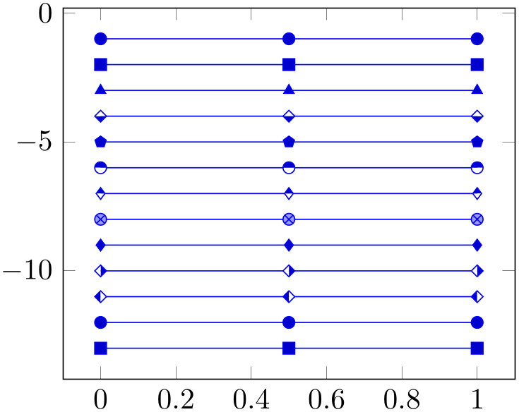
% Preamble: \pgfplotsset{width=7cm,compat=1.18}\begin{tikzpicture}\begin{axis}[stack plots=y,stack dir=minus,cycle list name=mark list*,]\addplot+ [blue] coordinates {(0,1) (0.5,1) (1,1)};\addplot+ [blue] coordinates {(0,1) (0.5,1) (1,1)};\addplot+ [blue] coordinates {(0,1) (0.5,1) (1,1)};\addplot+ [blue] coordinates {(0,1) (0.5,1) (1,1)};\addplot+ [blue] coordinates {(0,1) (0.5,1) (1,1)};\addplot+ [blue] coordinates {(0,1) (0.5,1) (1,1)};\addplot+ [blue] coordinates {(0,1) (0.5,1) (1,1)};\addplot+ [blue] coordinates {(0,1) (0.5,1) (1,1)};\addplot+ [blue] coordinates {(0,1) (0.5,1) (1,1)};\addplot+ [blue] coordinates {(0,1) (0.5,1) (1,1)};\addplot+ [blue] coordinates {(0,1) (0.5,1) (1,1)};\addplot+ [blue] coordinates {(0,1) (0.5,1) (1,1)};\addplot+ [blue] coordinates {(0,1) (0.5,1) (1,1)};\end{axis}\end{tikzpicture}Similar to mark list, the mark list* always employs the current color, but it doesn’t define one (see above for the \addplot+).
-
• color list (from top to bottom)
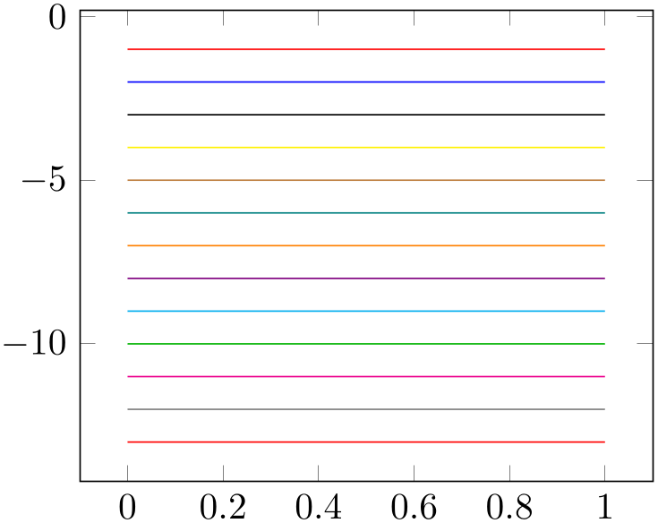
% Preamble: \pgfplotsset{width=7cm,compat=1.18}\begin{tikzpicture}\begin{axis}[stack plots=y,stack dir=minus,cycle list name=color list,]\addplot coordinates {(0,1) (0.5,1) (1,1)};\addplot coordinates {(0,1) (0.5,1) (1,1)};\addplot coordinates {(0,1) (0.5,1) (1,1)};\addplot coordinates {(0,1) (0.5,1) (1,1)};\addplot coordinates {(0,1) (0.5,1) (1,1)};\addplot coordinates {(0,1) (0.5,1) (1,1)};\addplot coordinates {(0,1) (0.5,1) (1,1)};\addplot coordinates {(0,1) (0.5,1) (1,1)};\addplot coordinates {(0,1) (0.5,1) (1,1)};\addplot coordinates {(0,1) (0.5,1) (1,1)};\addplot coordinates {(0,1) (0.5,1) (1,1)};\addplot coordinates {(0,1) (0.5,1) (1,1)};\addplot coordinates {(0,1) (0.5,1) (1,1)};\end{axis}\end{tikzpicture}The cycle list name=color choice also employs markers whereas color list uses only colors.
-
• linestyles (from top to bottom)
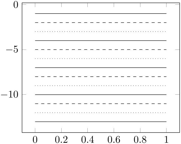
% Preamble: \pgfplotsset{width=7cm,compat=1.18}\begin{tikzpicture}\begin{axis}[stack plots=y,stack dir=minus,cycle list name=linestyles,]\addplot coordinates {(0,1) (0.5,1) (1,1)};\addplot coordinates {(0,1) (0.5,1) (1,1)};\addplot coordinates {(0,1) (0.5,1) (1,1)};\addplot coordinates {(0,1) (0.5,1) (1,1)};\addplot coordinates {(0,1) (0.5,1) (1,1)};\addplot coordinates {(0,1) (0.5,1) (1,1)};\addplot coordinates {(0,1) (0.5,1) (1,1)};\addplot coordinates {(0,1) (0.5,1) (1,1)};\addplot coordinates {(0,1) (0.5,1) (1,1)};\addplot coordinates {(0,1) (0.5,1) (1,1)};\addplot coordinates {(0,1) (0.5,1) (1,1)};\addplot coordinates {(0,1) (0.5,1) (1,1)};\addplot coordinates {(0,1) (0.5,1) (1,1)};\end{axis}\end{tikzpicture} -
• linestyles* contains more dotted line styles than linestyles (from top to bottom)
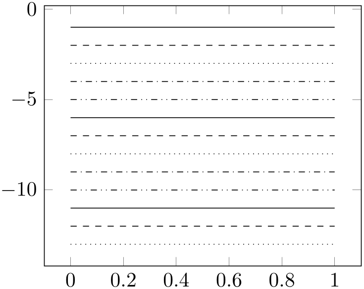
% Preamble: \pgfplotsset{width=7cm,compat=1.18}\begin{tikzpicture}\begin{axis}[stack plots=y,stack dir=minus,cycle list name=linestyles*,]\addplot coordinates {(0,1) (0.5,1) (1,1)};\addplot coordinates {(0,1) (0.5,1) (1,1)};\addplot coordinates {(0,1) (0.5,1) (1,1)};\addplot coordinates {(0,1) (0.5,1) (1,1)};\addplot coordinates {(0,1) (0.5,1) (1,1)};\addplot coordinates {(0,1) (0.5,1) (1,1)};\addplot coordinates {(0,1) (0.5,1) (1,1)};\addplot coordinates {(0,1) (0.5,1) (1,1)};\addplot coordinates {(0,1) (0.5,1) (1,1)};\addplot coordinates {(0,1) (0.5,1) (1,1)};\addplot coordinates {(0,1) (0.5,1) (1,1)};\addplot coordinates {(0,1) (0.5,1) (1,1)};\addplot coordinates {(0,1) (0.5,1) (1,1)};\end{axis}\end{tikzpicture} -
• auto The cycle list name=auto always denotes the most recently used cycle list activated by cycle list or cycle list name.
The definitions of all predefined cycle lists follow (see the end of this paragraph for a syntax description).
\pgfplotscreateplotcyclelist{color}{
blue,every mark/.append style={fill=blue!80!black},mark=*\\
red,every mark/.append style={fill=red!80!black},mark=square*\\
brown!60!black,every mark/.append style={fill=brown!80!black},mark=otimes*\\
black,mark=star\\
blue,every mark/.append style={fill=blue!80!black},mark=diamond*\\
red,densely dashed,every mark/.append style={solid,fill=red!80!black},mark=*\\
brown!60!black,densely dashed,every mark/.append style={
solid,fill=brown!80!black},mark=square*\\
black,densely dashed,every mark/.append style={solid,fill=gray},mark=otimes*\\
blue,densely dashed,mark=star,every mark/.append style=solid\\
red,densely dashed,every mark/.append style={solid,fill=red!80!black},mark=diamond*\\
}
\pgfplotscreateplotcyclelist{black white}{
every mark/.append style={fill=gray},mark=*\\
every mark/.append style={fill=gray},mark=square*\\
every mark/.append style={fill=gray},mark=otimes*\\
mark=star\\
every mark/.append style={fill=gray},mark=diamond*\\
densely dashed,every mark/.append style={solid,fill=gray},mark=*\\
densely dashed,every mark/.append style={solid,fill=gray},mark=square*\\
densely dashed,every mark/.append style={solid,fill=gray},mark=otimes*\\
densely dashed,every mark/.append style={solid},mark=star\\
densely dashed,every mark/.append style={solid,fill=gray},mark=diamond*\\
}
\pgfplotscreateplotcyclelist{exotic}{
teal,every mark/.append style={fill=teal!80!black},mark=*\\
orange,every mark/.append style={fill=orange!80!black},mark=square*\\
cyan!60!black,every mark/.append style={fill=cyan!80!black},mark=otimes*\\
red!70!white,mark=star\\
lime!80!black,every mark/.append style={fill=lime},mark=diamond*\\
red,densely dashed,every mark/.append style={solid,fill=red!80!black},mark=*\\
yellow!60!black,densely dashed,
every mark/.append style={solid,fill=yellow!80!black},mark=square*\\
black,every mark/.append style={solid,fill=gray},mark=otimes*\\
blue,densely dashed,mark=star,every mark/.append style=solid\\
red,densely dashed,every mark/.append style={solid,fill=red!80!black},mark=diamond*\\
}
% note that "." is the currently defined Tikz color.
\pgfplotscreateplotcyclelist{mark list}{
every mark/.append style={solid,fill=\pgfplotsmarklistfill},mark=*\\
every mark/.append style={solid,fill=\pgfplotsmarklistfill},mark=square*\\
every mark/.append style={solid,fill=\pgfplotsmarklistfill},mark=triangle*\\
every mark/.append style={solid},mark=star\\
every mark/.append style={solid,fill=\pgfplotsmarklistfill},mark=diamond*\\
every mark/.append style={solid,fill=\pgfplotsmarklistfill!40},mark=otimes*\\
every mark/.append style={solid},mark=|\\
every mark/.append style={solid,fill=\pgfplotsmarklistfill},mark=pentagon*\\
every mark/.append style={solid},mark=text,text mark=p\\
every mark/.append style={solid},mark=text,text mark=a\\
}
In this context, a common fill color expression can be customized using mark list fill:
-
/pgfplots/mark list fill={
color} (initially .!80!black)
Allows to customize the fill color for the mark list and mark list*.
For example, if you have black as color, the alternative choice mark list fill=.!50!white will produce much better results.
-
\pgfplotsmarklistfill 
Expands to \pgfkeysvalueof{/pgfplots/mark list fill}.
% note that "." is the currently defined Tikz color.
\pgfplotscreateplotcyclelist{mark list*}{
every mark/.append style={solid,fill=\pgfplotsmarklistfill},mark=*\\
every mark/.append style={solid,fill=\pgfplotsmarklistfill},mark=square*\\
every mark/.append style={solid,fill=\pgfplotsmarklistfill},mark=triangle*\\
every mark/.append style={solid,fill=\pgfplotsmarklistfill},mark=halfsquare*\\
every mark/.append style={solid,fill=\pgfplotsmarklistfill},mark=pentagon*\\
every mark/.append style={solid,fill=\pgfplotsmarklistfill},mark=halfcircle*\\
every mark/.append style={solid,fill=\pgfplotsmarklistfill,rotate=180},mark=halfdiamond*\\
every mark/.append style={solid,fill=\pgfplotsmarklistfill!40},mark=otimes*\\
every mark/.append style={solid,fill=\pgfplotsmarklistfill},mark=diamond*\\
every mark/.append style={solid,fill=\pgfplotsmarklistfill},mark=halfsquare right*\\
every mark/.append style={solid,fill=\pgfplotsmarklistfill},mark=halfsquare left*\\
}
\pgfplotscreateplotcyclelist{linestyles}{solid,dashed,dotted}
\pgfplotscreateplotcyclelist{linestyles*}{solid,dashed,dotted,dashdotted,dashdotdotted}
40 In an early version, these lists were called \coloredplotspeclist and \blackwhiteplotspeclist which appeared to be unnecessarily long, so they have been renamed. The old names are still accepted, however.
4.7.7.2Defining Own Cycle Lists
The second choice for cycle lists is to provide each entry directly as argument to cycle list,
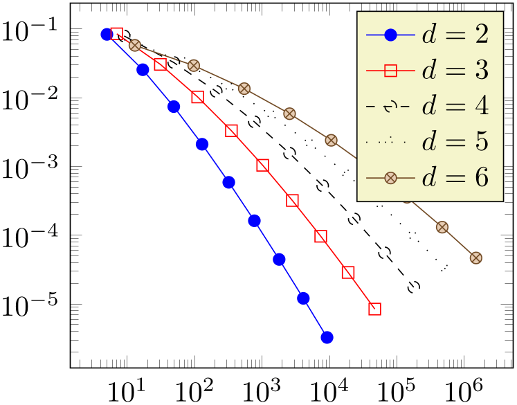
% Preamble: \pgfplotsset{width=7cm,compat=1.18}
\begin{tikzpicture}
\begin{loglogaxis}[
cycle list={
{blue,mark=*},
{red,mark=square},
{dashed,mark=o},
{loosely dotted,mark=+},
{brown!60!black,mark=otimes*,
mark options={fill=brown!40},
}% <-- don't add a comma here
},
]
\plotcoords
\legend{$d=2$,$d=3$,$d=4$,$d=5$,$d=6$}
\end{loglogaxis}
\end{tikzpicture}
(This example list requires \usetikzlibrary{plotmarks}).
The input format is described below in more detail.
4.7.7.3Defining and Labeling Own Cycle Lists
The last method for cycle lists is to combine the define named cycle lists in the preamble and use them with ‘cycle list name’:
-
\pgfplotscreateplotcyclelist{
name}{list}
\pgfplotscreateplotcyclelist{mylist}{
{blue,mark=*},
{red,mark=square},
{dashed,mark=o},
{loosely dotted,mark=+},
{brown!60!black,mark options={fill=brown!40},mark=otimes*}% <-- don't add a comma here
}
...
\begin{axis}[cycle list name=mylist]
...
\end{axis}
4.7.7.4Defining Cycle Lists: Input Format
A cycle list is defined by key–value pairs of sorts
cycle list={list} or by the equivalent macro outlined above,
\pgfplotscreateplotcyclelist{name}{list}.
In this context, the argument
list
is usually a comma separated list of lists of style keys like colors, line styles, marker types and marker styles. This
“comma list of comma lists” structure requires to encapsulate the inner list using curly braces:
\pgfplotscreateplotcyclelist{mylist}{
{blue,mark=*},
{red,mark=square},
{dashed,mark=o},
{loosely dotted,mark=+},
{brown!60!black,mark options={fill=brown!40},mark=otimes*}% <-- don't add a comma here
}
Alternatively, one can terminate the inner lists (i.e. those for one single plot) with ‘\\’:
\begin{axis}[
cycle list={
blue,mark=*\\
red,mark=square\\
dashed,mark=o\\
loosely dotted,mark=+\\
brown!60!black,mark options={fill=brown!40},mark=otimes*\\
},
]
...
\end{axis}
In this case, the last entry also needs a terminating ‘\\’, but one can omit braces around the single entries.
4.7.7.5Manipulating Associations of Cycle Lists to Plots
-
/pgfplots/cycle list shift={
integer} (initially empty)
Allows to shift the index into the
cycle list. If
integer
is \(n\), the list element \(i+n\) will be taken instead of the \(i\)th one. Remember that \(i\) is the index of the
current \addplot command (starting with \(0\)).
Since a cycle list is queried immediately when \addplot (or \addplot+) is called, you can adjust the cycle list shift for selected plots:
If the result is negative, \(i+n <0\), the list index \(-(i+n)\) will be taken. For example, cycle list shift=-10 and \(i<10\) will result in list index \(10-i\). Note that you can use reverse legend to reverse legends, so this feature is probably never needed.
4.7.7.6Defining Cycle Lists based on Color Maps
In addition to defining cycle lists from scratch, pgfplots supports dedicated input definitions of
cycle list=list
which allow to acquire values from an existing colormap. In this case,
list
contains keys enclosed in square brackets:
The first syntax, of colormap, allows to convert the colors of a colormap to a cycle list. It can be specified without argument by means of cycle list={[of colormap]} in order to take the value of the most recently assigned colormap name (i.e. the current colormap). It can also be specified as cycle list={[of colormap=name]} in which case it will use the specified colormap name=name. In both cases, the definition merely converts the colors as they are found in the colormap into the cycle list, i.e. there is no interpolation involved. Applying this to the default colormap name=hot which has \(4\) colors results in the following example:
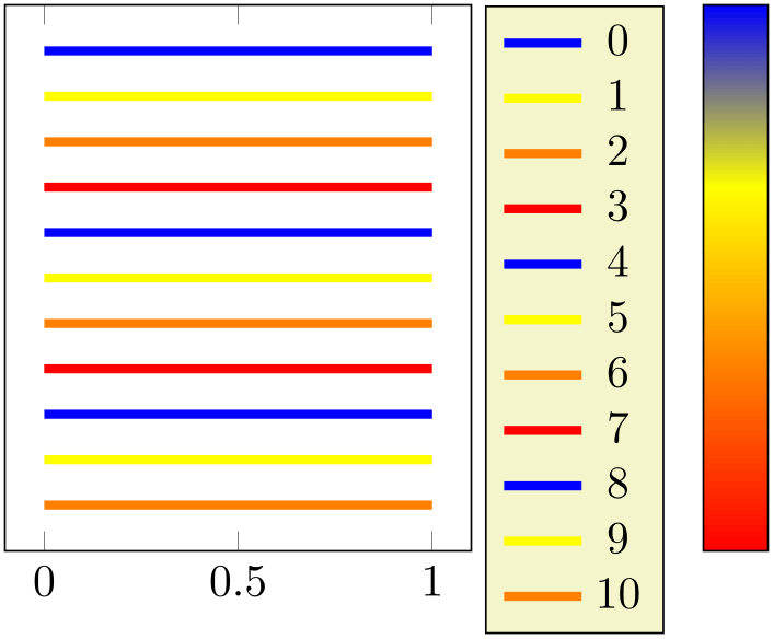
% Preamble: \pgfplotsset{width=7cm,compat=1.18}
\begin{tikzpicture}
\begin{axis}[
colormap name=hot,colorbar,
cycle list={[of colormap]},
%
cycle from colormap manual style,
]
                          \addplot coordinates
                      {(0,1) (0.5,1) (1,1)};
                          \addplot coordinates
                      {(0,1) (0.5,1) (1,1)};
                          \addplot coordinates
                      {(0,1) (0.5,1) (1,1)};
                          \addplot coordinates
                      {(0,1) (0.5,1) (1,1)};
                          \addplot coordinates
                      {(0,1) (0.5,1) (1,1)};
                          \addplot coordinates
                      {(0,1) (0.5,1) (1,1)};
                          \addplot coordinates
                      {(0,1) (0.5,1) (1,1)};
                          \addplot coordinates
                      {(0,1) (0.5,1) (1,1)};
                          \addplot coordinates
                      {(0,1) (0.5,1) (1,1)};
                          \addplot coordinates
                      {(0,1) (0.5,1) (1,1)};
                          \addplot coordinates
                      {(0,1) (0.5,1) (1,1)};
\end{axis}
\end{tikzpicture}
Note that since hot has \(4\) colors, the cycle list also contains \(4\) entries which are repeated every \(4\) plots.
The second possibility resembles samples of colormap: it expects samples of colormap={number} of colormap name. It chooses
number
samples of the selected colormap.
The third possibility is similar to color of colormap: it expects colors of colormap={list} or colors of colormap={list} of colormap name. This choice interpolates colors and expects a
list
of values in the range \([0,1000]\) where \(0\) is the lowest element in the
colormap and \(1000\) is its highest element:
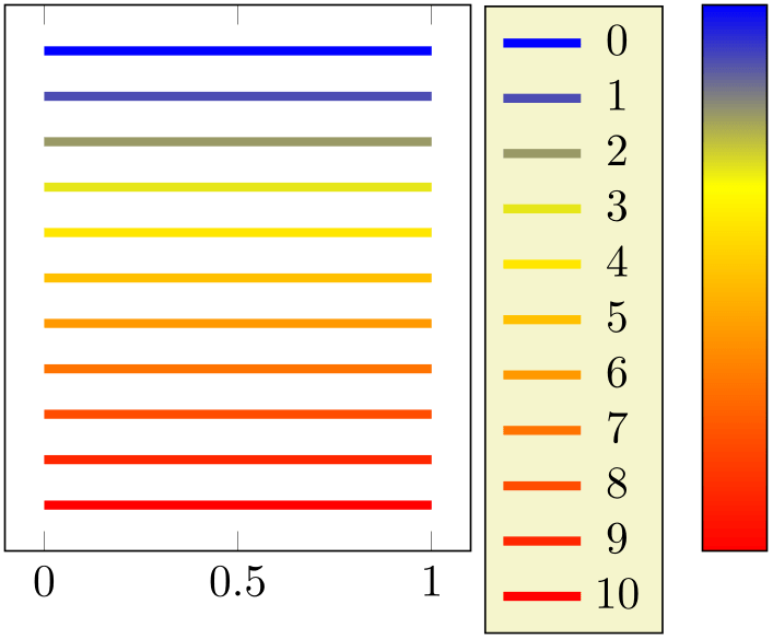
% Preamble: \pgfplotsset{width=7cm,compat=1.18}
\begin{tikzpicture}
\begin{axis}[
colormap name=hot,colorbar,
cycle list={
[colors of colormap={0,100,...,1000}]},
%
cycle from colormap manual style,
]
                          \addplot coordinates
                      {(0,1) (0.5,1) (1,1)};
                          \addplot coordinates
                      {(0,1) (0.5,1) (1,1)};
                          \addplot coordinates
                      {(0,1) (0.5,1) (1,1)};
                          \addplot coordinates
                      {(0,1) (0.5,1) (1,1)};
                          \addplot coordinates
                      {(0,1) (0.5,1) (1,1)};
                          \addplot coordinates
                      {(0,1) (0.5,1) (1,1)};
                          \addplot coordinates
                      {(0,1) (0.5,1) (1,1)};
                          \addplot coordinates
                      {(0,1) (0.5,1) (1,1)};
                          \addplot coordinates
                      {(0,1) (0.5,1) (1,1)};
                          \addplot coordinates
                      {(0,1) (0.5,1) (1,1)};
                          \addplot coordinates
                      {(0,1) (0.5,1) (1,1)};
\end{axis}
\end{tikzpicture}
In this case, we specified \(11\) colors and have \(11\) plots. Clearly, interpolated colors are of limited use and are only applicable for special use cases. Use only cycle lists of this sort if the colormap allows a suitable distinction of adjacent plot lines! Note that colors of colormap is quite similar to the related way to build colormaps based on existing colormaps as outlined in Section 4.7.6.4 on page (page for section 4.7.6.4).
A related choice is indices of colormap={list}. As above, it accepts an optional ‘of’ clause of the form
indices of colormap={list} of colormap name. The main argument is a list of indices \(0\le N_i < N\) where \(N\) is the number colors in the colormap definition
(compare the documentation of index of colormap). Indices which are out of range are clipped to the nearest index. For example, viridis comes with
\(\pgfplotscolormapsizeof {viridis}\) elements and we can write
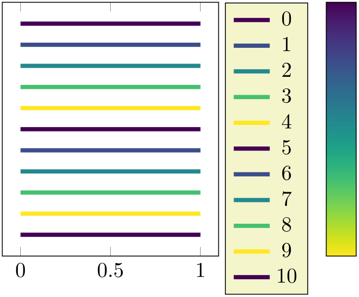
% Preamble: \pgfplotsset{width=7cm,compat=1.18}
\begin{tikzpicture}
\begin{axis}[
colormap name=viridis,colorbar,
cycle list={
[indices of colormap={0,4,8,12,17} of viridis]},
%
cycle from colormap manual style,
]
                          \addplot coordinates
                      {(0,1) (0.5,1) (1,1)};
                          \addplot coordinates
                      {(0,1) (0.5,1) (1,1)};
                          \addplot coordinates
                      {(0,1) (0.5,1) (1,1)};
                          \addplot coordinates
                      {(0,1) (0.5,1) (1,1)};
                          \addplot coordinates
                      {(0,1) (0.5,1) (1,1)};
                          \addplot coordinates
                      {(0,1) (0.5,1) (1,1)};
                          \addplot coordinates
                      {(0,1) (0.5,1) (1,1)};
                          \addplot coordinates
                      {(0,1) (0.5,1) (1,1)};
                          \addplot coordinates
                      {(0,1) (0.5,1) (1,1)};
                          \addplot coordinates
                      {(0,1) (0.5,1) (1,1)};
                          \addplot coordinates
                      {(0,1) (0.5,1) (1,1)};
\end{axis}
\end{tikzpicture}
Note that ‘ of viridis’ is actually redundant as viridis was already selected in this case.
The complete syntax on how to customize of colormap is the same as the building blocks to define colormaps based on other colormaps as described in Section 4.7.6.4 on page (page for section 4.7.6.4) – with the difference that cycle list={[of colormap]} inserts the selected colors into the cycle list instead of a colormap.
Note that all these special lists are valid arguments for \pgfplotscreateplotcyclelist and can also appear as sublists in cycle multi list and its variants.
Since creating a cycle list from a colormap necessarily results in plots without markers and line style variations, it makes sense to combine the result with cycle multiindex* list, i.e. to join two existing lists. The following example joins a pure color list with markers:
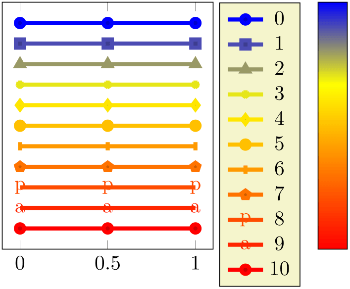
% Preamble: \pgfplotsset{width=7cm,compat=1.18}
\begin{tikzpicture}
\begin{axis}[
colormap name=hot,colorbar,
cycle multiindex* list={
[samples of colormap=11]\nextlist
mark list\nextlist
},
cycle from colormap manual style,
]
                          \addplot coordinates
                      {(0,1) (0.5,1) (1,1)};
                          \addplot coordinates
                      {(0,1) (0.5,1) (1,1)};
                          \addplot coordinates
                      {(0,1) (0.5,1) (1,1)};
                          \addplot coordinates
                      {(0,1) (0.5,1) (1,1)};
                          \addplot coordinates
                      {(0,1) (0.5,1) (1,1)};
                          \addplot coordinates
                      {(0,1) (0.5,1) (1,1)};
                          \addplot coordinates
                      {(0,1) (0.5,1) (1,1)};
                          \addplot coordinates
                      {(0,1) (0.5,1) (1,1)};
                          \addplot coordinates
                      {(0,1) (0.5,1) (1,1)};
                          \addplot coordinates
                      {(0,1) (0.5,1) (1,1)};
                          \addplot coordinates
                      {(0,1) (0.5,1) (1,1)};
\end{axis}
\end{tikzpicture}
Please refer to the next subsection for details about cycle multiindex* list.
Note that the preceding examples all use the following style.
-
/pgfplots/cycle from colormap manual style(style, no value) 
A style defined in this manual. It has the value
\pgfplotsset{
cycle from colormap manual style/.style={
x=3cm,y=10pt,ytick=\empty,
colorbar style={x=,y=,ytick=\empty},
point meta min=0,point meta max=1,
stack plots=y,
y dir=reverse,colorbar style={y dir=reverse},
every axis plot/.style={line width=2pt},
legend entries={0,...,20},
legend pos=outer north east,
},
}
It is possible to call
\pgfplotsset{cycle list={a list}} or cycle list name
between plots. Such a setting remains effective until the end of the current
TeX
group (that means curly braces). Every \addplot command
queries the cycle list using the plot index; it
doesn’t hurt if cycle lists have changed in the meantime.
-
/pgfplots/cycle list/.define={
name}{list}
A command which merely
calls \pgfplotscreateplotcyclelist{name}{list} without actually selecting it as the current list.
Note that pgfplots uses this to implement its cycle list key as follows:
\pgfplotsset{
cycle list/.style={%
cycle list/.define={@internal@}{#1},%
cycle list name={@internal@}%
},
}
4.7.7.7Building Block to Combine Different Cycle Lists
The following keys allow to combined different cycle lists in order to build more complex ones.
-
/pgfplots/cycle multi list=
list 1\nextlistlist 2\nextlist\(\ldots \)
This is one of two ways to employ more than one cycle list in order to determine the plot style (see also cycle multiindex list for the other one). This is probably best explained using an example:
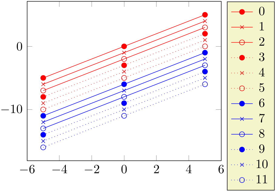
% Preamble: \pgfplotsset{width=7cm,compat=1.18}
\begin{tikzpicture}
\begin{axis}[
cycle multi list={
red,blue\nextlist
                                solid,{dotted,mark
                    options={solid}}\nextlist
mark=*,mark=x,mark=o
},
samples=3,
legend entries={0,...,20},
legend pos=outer north east,
]
\addplot {x};
\addplot {x-1};
\addplot {x-2};
\addplot {x-3};
\addplot {x-4};
\addplot {x-5};
\addplot {x-6};
\addplot {x-7};
\addplot {x-8};
\addplot {x-9};
\addplot {x-10};
\addplot {x-11};
\end{axis}
\end{tikzpicture}
The provided cycle multi list consists of three lists. The style for a single plot is made up using elements of each of the three lists: the first plot has style red,solid,mark=*, the second has red,solid,mark=x, the third has red,solid,mark=o. The fourth plot restarts the third list and uses the next one of list \(2\): it has red,dotted,mark options={solid},mark=* and so on.
The last list will always be advanced for a new plot. The list before the last (in our case the second list) will be advanced after the last one has been reset. In other words: cycle multi list allows a composition of different cycle list in a lexicographical way.41
The argument for cycle multi list is a sequence
of arguments as they would have been provided for
cycle list, separated by \nextlist. In addition to providing a new cycle list, the
list \(i\)
elements can also denote cycle list name values
(including the special auto cycle list which is the most recently
assigned cycle list or
cycle list name). The final \nextlist is optional.
The list in our example above could have been written as
\begin{axis}[
cycle multi list={
red\\blue\\\nextlist
solid\\dotted,mark options={solid}\\\nextlist
mark=*\\mark=x\\mark=o\\
},
]
as well (note the terminating \\ commands!).
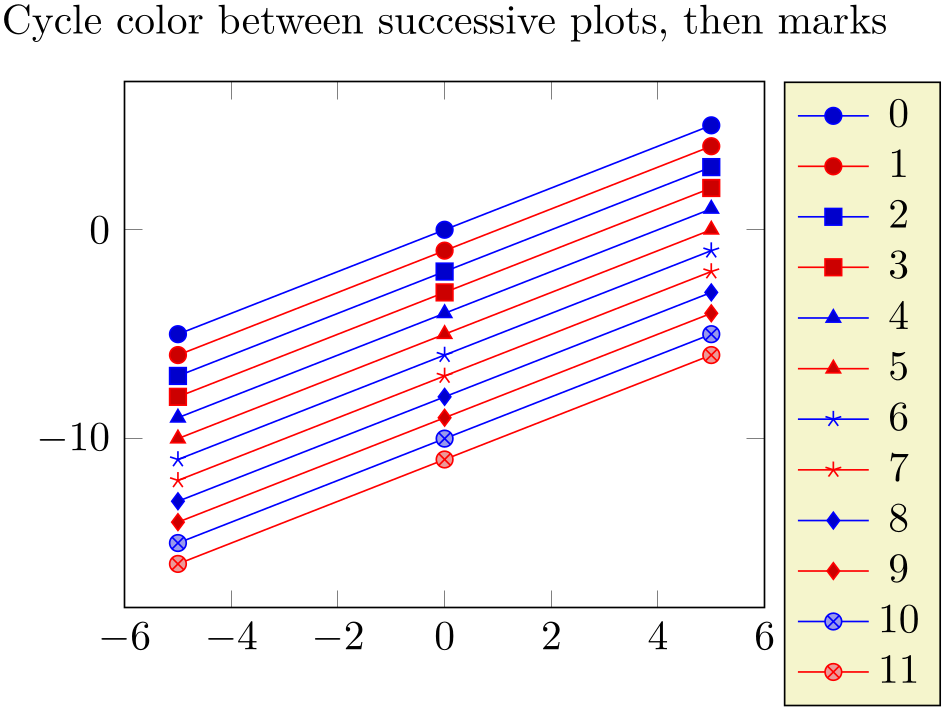
% Preamble: \pgfplotsset{width=7cm,compat=1.18}
\begin{tikzpicture}
\begin{axis}[
title={Cycle color between successive plots, then marks},
cycle multi list={
mark list\nextlist
blue,red
},
samples=3,
legend entries={0,...,20},
legend pos=outer north east,
]
\addplot {x};
\addplot {x-1};
\addplot {x-2};
\addplot {x-3};
\addplot {x-4};
\addplot {x-5};
\addplot {x-6};
\addplot {x-7};
\addplot {x-8};
\addplot {x-9};
\addplot {x-10};
\addplot {x-11};
\end{axis}
\end{tikzpicture}
The
list \(i\)
entry can also contain just the first \(n\) elements of an already known cycle list name using the syntax [number of]cycle list name. For example [2 of]mark list will use the first \(2\) elements of
mark list:
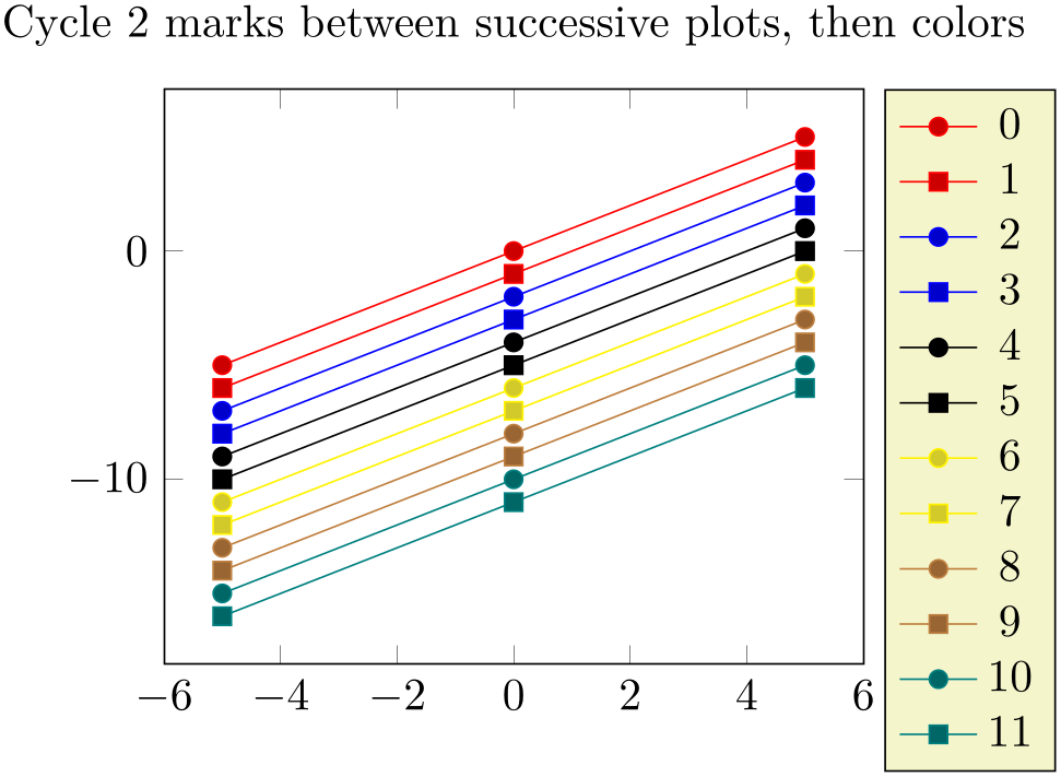
% Preamble: \pgfplotsset{width=7cm,compat=1.18}
\begin{tikzpicture}
\begin{axis}[
title={Cycle 2 marks between successive plots, then colors},
cycle multi list={
                              color
                  list\nextlist
[2 of]mark list
},
samples=3,
legend entries={0,...,20},
legend pos=outer north east,
]
\addplot {x};
\addplot {x-1};
\addplot {x-2};
\addplot {x-3};
\addplot {x-4};
\addplot {x-5};
\addplot {x-6};
\addplot {x-7};
\addplot {x-8};
\addplot {x-9};
\addplot {x-10};
\addplot {x-11};
\end{axis}
\end{tikzpicture}
-
/pgfplots/cycle multiindex list=
list 1\nextlistlist 2\nextlist\(\ldots \)
This is one of two ways to employ more than one cycle list in order to determine the plot style (see also cycle multi list for the other one). The difference between the two choices is how the list index is mapped into the sub lists. Let us start with our example:
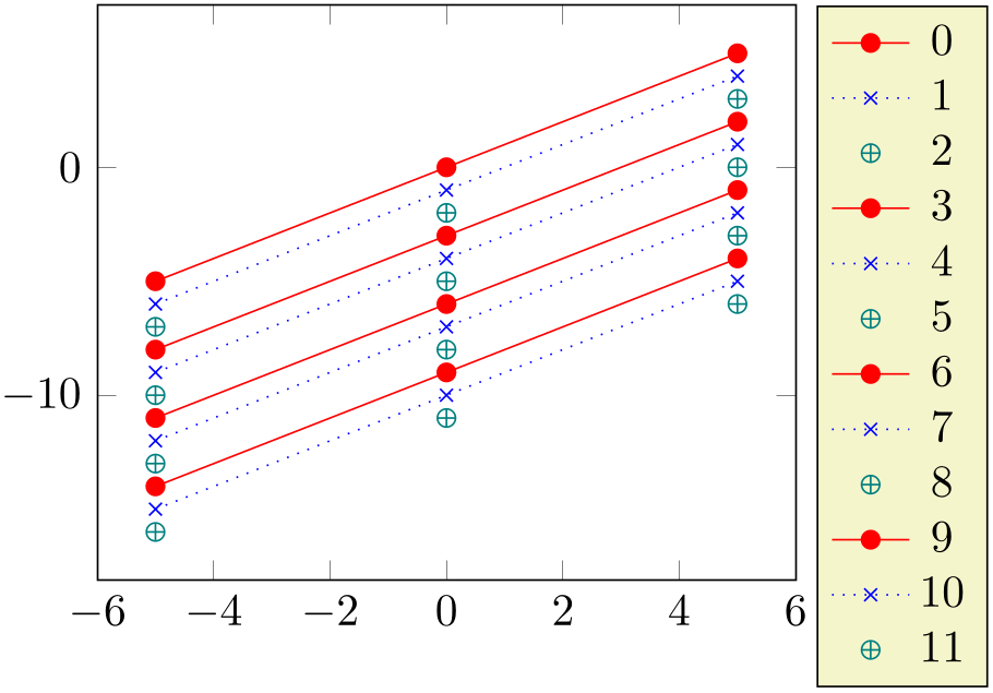
% Preamble: \pgfplotsset{width=7cm,compat=1.18}
\begin{tikzpicture}
\begin{axis}[
cycle multiindex list={
red,blue,teal\nextlist
                                solid\\dotted,mark
                    options={solid}\\only marks\\\nextlist
mark=*,mark=x,mark=oplus\nextlist
},
samples=3,
legend entries={0,...,20},
legend pos=outer north east,
]
\addplot {x};
\addplot {x-1};
\addplot {x-2};
\addplot {x-3};
\addplot {x-4};
\addplot {x-5};
\addplot {x-6};
\addplot {x-7};
\addplot {x-8};
\addplot {x-9};
\addplot {x-10};
\addplot {x-11};
\end{axis}
\end{tikzpicture}
The provided cycle multiindex list consists of three lists. The style for a single plot is made up using elements of each of the three lists: the first plot has style red,solid,mark=*, the second has blue,dotted,mark options={solid},mark=x, the third has teal,only marks,oplus. The fourth plot restarts all lists and uses the same as the first plot, i.e. red,solid,mark=*.
Note that the second list uses the list-separator ‘\\’ which requires a final terminator as defined for cycle list.
Thus, this style uses the same index into every list (a “multi index”). Consequently, it has considerably less different choices than cycle multi list (which results in all possible variations), but its combination method addresses different use cases.
The argument for cycle multiindex list has the very same format as the one for cycle multi list, including the special [2 of]mark list syntax and providing other cycle lists by name:
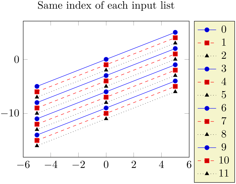
% Preamble: \pgfplotsset{width=7cm,compat=1.18}
\begin{tikzpicture}
\begin{axis}[
title={Same index of each input list},
cycle multiindex list={
[3 of]mark list\nextlist
blue,red\nextlist
linestyles\nextlist
},
samples=3,
legend entries={0,...,20},
legend pos=outer north east,
]
\addplot {x};
\addplot {x-1};
\addplot {x-2};
\addplot {x-3};
\addplot {x-4};
\addplot {x-5};
\addplot {x-6};
\addplot {x-7};
\addplot {x-8};
\addplot {x-9};
\addplot {x-10};
\addplot {x-11};
\end{axis}
\end{tikzpicture}
Note that cycle multiindex list accepts lists of different sizes. The size of a cycle multiindex list is the size of the largest input list, all smaller input lists are padded with empty option lists. That is why the previous example uses the color black for every third plot: there is no color in the second list, and omitting the color results in black. As soon as the last item of the largest sublist has been used, the list is restarted.
-
/pgfplots/cycle multiindex* list=
list 1\nextlistlist 2\nextlist\(\ldots \)
A variant of cycle multiindex list which behaves in the same way – except for sublists of different sizes.
As documented above, the unstarred version cycle multiindex list pads missing entries with empty options lists until all list elements have the same size.
The starred key cycle multiindex* list restarts sublists independently whenever they reach their end:

% Preamble: \pgfplotsset{width=7cm,compat=1.18}
\begin{tikzpicture}
\begin{axis}[
title={Same index of each input list, lists restarted},
cycle multiindex* list={
[3 of]mark list\nextlist
blue,red\nextlist
linestyles\nextlist
},
samples=3,
legend entries={0,...,20},
legend pos=outer north east,
]
\addplot {x};
\addplot {x-1};
\addplot {x-2};
\addplot {x-3};
\addplot {x-4};
\addplot {x-5};
\addplot {x-6};
\addplot {x-7};
\addplot {x-8};
\addplot {x-9};
\addplot {x-10};
\addplot {x-11};
\end{axis}
\end{tikzpicture}
This is the very same example as documented for the unstarred variant cycle multiindex list. However, the second sublist has fewer elements – and while the unstarred variant resulted in black, the starred variant restarts the second sublist as soon as its two existing colors are consumed.
This style allows to concatenate lists in complex ways:
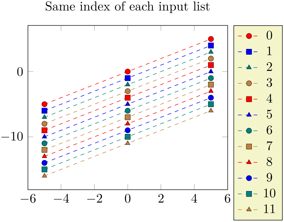
% Preamble: \pgfplotsset{width=7cm,compat=1.18}
\begin{tikzpicture}
\begin{axis}[
title={Same index of each input list},
cycle multiindex* list={
red,blue,teal,brown\nextlist
mark=*,mark=square*,mark=triangle*\nextlist
dashed,every mark/.append style={
solid,draw=.!50!black,fill=.,}\\
\nextlist
},
samples=3,
legend entries={0,...,20},
legend pos=outer north east,
]
\addplot {x};
\addplot {x-1};
\addplot {x-2};
\addplot {x-3};
\addplot {x-4};
\addplot {x-5};
\addplot {x-6};
\addplot {x-7};
\addplot {x-8};
\addplot {x-9};
\addplot {x-10};
\addplot {x-11};
\end{axis}
\end{tikzpicture}
We see that the four different colors appear periodically as expected. We also see the three different markers with their own period (which restarts every fourth plot as expected). But the third sublist contains just one element as we can see by its separator character ‘\\’ which appears just once at the end of the list! Consequently, this list is restarted for every plot such that every plot receives its arguments.
41 For those who prefer formulas: The plot with index \(0 \le i < N\) will use cycle list offsets \(i_0,i_1,\dotsc ,i_k\), \(0 \le i_m < N_m\) where \(k\) is the number of arguments provided to cycle multi list and \(N_m\) is the number of elements in the \(m\)th cycle list. The offsets \(i_m\) are computed in a loop { int tmp=i; for( int m=k-1; m>=0; m=m-1 ) { i_m = tmp%N_m; tmp = tmp/N_m; }}.
4.7.8Axis Background
-
/pgfplots/axis background(initially empty) 
This is a style to configure the appearance of the axis
as such. It can be defined and/or changed using the
axis background/.style={options} method. A background path will be generated with
options, which may contain fill colors or shadings.
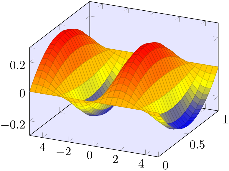
% Preamble: \pgfplotsset{width=7cm,compat=1.18}
\begin{tikzpicture}
\begin{axis}[
axis background/.style={fill=blue!10},
]
\addplot3 [
surf,
y domain=0:1,
]
{sin(deg(x)) * y*(1-y)};
\end{axis}
\end{tikzpicture}
Please note that legends are filled with white in the default configuration.
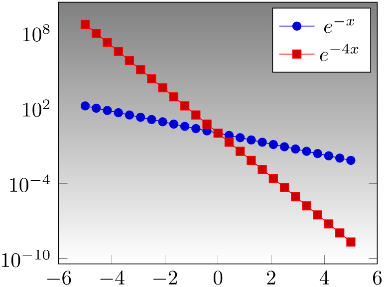
% Preamble: \pgfplotsset{width=7cm,compat=1.18}
\begin{tikzpicture}
\begin{semilogyaxis}[
axis background/.style={
shade,top color=gray,bottom color=white,
},
legend style={fill=white},
]
\addplot {exp(-x)};
\addplot {exp(-4*x)};
\legend{$e^{-x}$,$e^{-4x}$}
\end{semilogyaxis}
\end{tikzpicture}
Details about fill and shade can be found in the PGF/TikZ manual.