Manual for Package pgfplots
2D/3D Plots in LATeX, Version 1.18.2
https://github.com/pgf-tikz/pgfplots
The Reference
4.23Transforming Coordinate Systems
Usually, pgfplots works with Cartesian coordinates. However, one may want to provide coordinates in a different coordinate system.
In this case, the data cs key can be used to identify the input coordinate system:
-
/pgfplots/data cs=cart|polar|polarrad (initially cart) 
Defines the coordinate system (‘cs’) of the input coordinates. pgfplots will apply transformations if the argument does not match the expected coordinate system.
Use data cs if your input has a different coordinate system than the axis. More precisely, every axis type has its own coordinate system. For example, a normal axis has the cart coordinate system, whereas a polaraxis has a polar coordinate system. The use of data cs with a different argument than the default of your axis instructs pgfplots to apply transformations.
At the time of this writing, pgfplots supports the following values for data cs:
The data cs=cart denotes the Cartesian coordinate system. It is the coordinate system of the usual axis (or its logarithmic variants). It can have three components, \(x\), \(y\), and \(z\). Specifying it is only necessary if you have a non-Cartesian axis:

% Preamble: \pgfplotsset{width=7cm,compat=1.18}
% requires \usepgfplotslibrary{polar}
\begin{tikzpicture}
\begin{polaraxis}
                        \addplot coordinates
                    {(90,1) (180,1)};
                        \addplot+ [data cs=cart] coordinates
                    {
(1,0)
(0.5,0.5)
};
\end{polaraxis}
\end{tikzpicture}
The data cs=polar is the (two-dimensional) coordinate system with (angle, radius), i.e. the first component “\(x\)” is the angle and the second component “\(y\)” is the radius. The angle is a number in the periodic range \([0,360)\); the radius is any number. If a polar coordinate has a \(z\) component, it is taken as is (the transformations ignore it).
% Preamble: \pgfplotsset{width=7cm,compat=1.18}
\begin{tikzpicture}
\begin{axis}
\addplot+ [data cs=polar,domain=0:360] (\x,1);
\end{axis}
\end{tikzpicture}
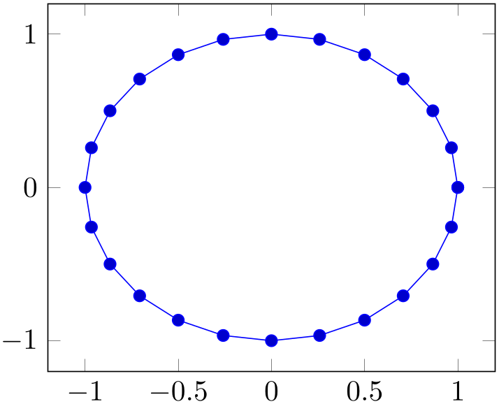
The data cs=polarrad is similar to polar, but it expects the angle in radians, i.e. in the periodic range \([0,2\pi )\).

% Preamble: \pgfplotsset{width=7cm,compat=1.18}
\begin{tikzpicture}
\begin{axis}
\addplot+ [data cs=polarrad,domain=0:2*pi] (\x,1);
\end{axis}
\end{tikzpicture}
Note that the math function deg( rad
rad ) transforms
rad
into degrees and rad(degree) transforms
degree
into radians. Consequently, polar and
polarrad are more or less equivalent for plot expression.
) transforms
rad
into degrees and rad(degree) transforms
degree
into radians. Consequently, polar and
polarrad are more or less equivalent for plot expression.

% Preamble: \pgfplotsset{width=7cm,compat=1.18}
\begin{tikzpicture}
\begin{axis}[
axis equal,
minor tick num=1,
]
\def\FREQUENCY{3}
\addplot [red,domain=0:360,samples=200,
smooth,data cs=polar]
(x,{30-8*sin(\FREQUENCY*x)});
\addplot [samples=40,domain=0:2*pi,dashed,
data cs=polar] (deg(x),30);
                    \addplot [mark=oplus,only marks] coordinates
                    {(0,0)};
\end{axis}
\end{tikzpicture}
At the point of this writing, the data cs method will work for most plot handlers. But for complicated plot handlers, further logic may be needed which is not yet available (for example, the quiver plot handler might not be able to convert its direction vectors correctly).70
-
\pgfplotsaxistransformcs{
fromname}{toname}
Expects the current point in a set of keys, provided in the coordinate
system
fromname
and replaces them by the same coordinates represented in
toname.
On input, the coordinates are stored in /data point/x, /data point/y, and /data point/z (the latter may be empty). The macro
will test if there is a declared coordinate transformation from
fromname
to
toname
and invoke it. If there is none, it will attempt to convert to
cart first and then from
cart to
toname. If that does not exist either, the operation fails.
-
\pgfplotsdefinecstransform{
fromname}{toname}{code}
Defines a new coordinate system transformation. The
code
is expected to get input and write output as described for
\pgfplotsaxistransformcs.
Implementing a new coordinate system immediately raises the question in which math mode the operations shall be applied. pgfplots supports different so-called “coordinate math systems” for generic operations, and for each individual coordinate as well. These coordinate math systems can either use basic pgf math arithmetics, the fpu, or perhaps there will come a LuaTeX library.
The documentation of this system is beyond the scope of this manual.71 Please consider reading the source code comments and the source of existing transformations if you intend to write own transformations.
70 In case you run into problems, consider writing a bug report or ask others in TeX online discussion forums.
71 Which is quite comprehensive even without API documentation, as you will certainly agree…
4.23.1Interaction of Transformations
There are a couple of coordinate mappings in pgfplots. For each encountered coordinate in a coordinate stream (\addplot), it applies the following steps:
-
1. Remember the “raw” coordinates in math constants rawx, rawy, rawz,
-
2. apply pre filter,
-
3. apply x coord trafo, logarithm if necessary, and x filter (in this order),
-
4. apply y coord trafo, logarithm if necessary, and y filter,
-
5. apply z coord trafo, logarithm if necessary, and z filter,
-
6. apply filter point,
-
7. transform from data cs to the coordinate system of axis type,
-
8. handle coordinate stacking (stack plots=x and/or stack plots=y).
Here, pre filter takes no arguments; it simply prepares the following filters. Consequently, the first item which actually accepts the input argument is x coord trafo. This method is part of the parsing; it accepts the “raw” coordinate which may be in symbolic form. The output of x coord trafo and its variants is a number. This number can be filtered or transformed by means of x filter and its variants. Note that x filter simply takes one argument: the result of x coord trafo.
The intended meaning of x coord trafo is to define how the “raw” string form as provided by the user makes its way into pgfplots. It is also the only transformation which has an inverse, the key x coord inv trafo. The inverse can be used to transform back from internal numeric form to some string for the end user. The key x coord trafo can only be defined as option to an axis, i.e. it it cannot be provided to \addplot.
The meaning of x filter and its variants is to transform numbers or to conditionally throw away numbers (and thus the entire coordinate). Each \addplot can receive its own (set of) filters.
The key filter point accepts all arguments (more precisely: the result of the preceding steps). It can rely on \(x\), \(y\), and \(z\), and it can change any of them. The way it accepts the coordinates is by means of keys /data point/x and its variants for \(y\) and \(z\). In principle, filter point is the most general filter. However, you can define both x filter and filter point, and both will be applied. Each \addplot can receive its own filter point.
The implementation for the key data cs is similar to filter point in that it accepts the result of all previous mapping steps. However, it maps from a well-defined input coordinate system to some well-defined internal coordinate system (which is inherent to the axis). Each \addplot can receive its own data cs.
Finally, stack plots takes measures to add/subtract the results. Stacking of plots is a property of the axis; it is not intended to be provided as argument to \addplot.72