Manual for Package pgfplots
2D/3D Plots in LATeX, Version 1.18.2
https://github.com/pgf-tikz/pgfplots
The Reference
4.17Custom Annotations
Often, one may want to add custom drawing elements or descriptive texts to an axis. These graphical elements should be associated to some logical coordinate, grid point, or perhaps they should just be placed somewhere into the axis.
pgfplots assists with the following ways when it comes to annotations:
-
1. You can explicitly provide any TikZ instruction like \draw ... ; into the axis. Here, the axis cs allows to provide coordinates of pgfplots.
Furthermore, rel axis cs allows to position TikZ elements relatively (like “\(50\%\) of the axis’ width).
-
2. pgfplots can automatically generate nodes at every coordinate using its nodes near coords feature.
-
3. pgfplots allows you to place nodes on a plot, using the \addplot ... node[pos=
 fraction
 ] {}; feature.
This section explains all of the approaches, except for the nodes near coords feature which is documented in its own section.
4.17.1Accessing Axis Coordinates in Graphical Elements
-
Coordinate system axis cs 
pgfplots provides a new coordinate system for use inside of an axis, the “axis coordinate system”, axis cs.
Note that this coordinate system is actually the default one whenever one writes graphical elements in an axis. There is just one place where you really need to provide this coordinate system explicitly: if you have symbolic x coords.
Consequently, you can refer to this documentation as reference only; most standard use cases work directly (as of compat=1.11).
It can be used to draw any TikZ graphics at axis coordinates. It is used like
% Preamble: \pgfplotsset{width=7cm,compat=1.18}
\tikzstyle{every pin}=[
fill=white,
draw=black,
font=\footnotesize,
]
\begin{tikzpicture}
\begin{loglogaxis}[
xlabel={\textsc{Dof}},
ylabel={$L_2$ Error},
]
                        \addplot coordinates
                    {
(11, 6.887e-02)
(71, 3.177e-02)
(351, 1.341e-02)
(1471, 5.334e-03)
(5503, 2.027e-03)
(18943, 7.415e-04)
(61183, 2.628e-04)
(187903, 9.063e-05)
(553983, 3.053e-05)
};
\node [coordinate,pin=above:{Bad!}]
at (axis cs:5503,2.027e-03) {};
\node [coordinate,pin=left:{Good!}]
at (axis cs:187903,9.063e-05) {};
\end{loglogaxis}
\end{tikzpicture}
However, since axis cs is the default coordinate system of pgfplots, you can simply omit the prefix axis cs: in coordinate descriptions.61
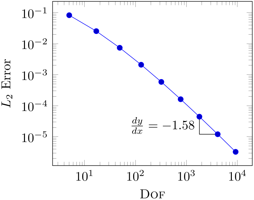
% Preamble: \pgfplotsset{width=7cm,compat=1.18}
\begin{tikzpicture}
\begin{loglogaxis}[
xlabel=\textsc{Dof},
ylabel=$L_2$ Error,
]
\draw
(1793,4.442e-05)
|- (4097,1.207e-05)
node [near start,left]
                                    {$\frac{dy}{dx} =
                    -1.58$};
                        \addplot coordinates
                    {
(5, 8.312e-02)
(17, 2.547e-02)
(49, 7.407e-03)
(129, 2.102e-03)
(321, 5.874e-04)
(769, 1.623e-04)
(1793, 4.442e-05)
(4097, 1.207e-05)
(9217, 3.261e-06)
};
\end{loglogaxis}
\end{tikzpicture}
The effect of axis cs is to apply any custom transformations (including symbolic x coords), logarithms, data scaling transformations or whatever pgfplots usually does and provides a low level pgf coordinate as result.
In case you need only one component (say, the \(y\) component) of such a vector, you can use the \pgfplotstransformcoordinatey command, see Section 9.4 for details about basic level access.
The result of axis cs is always an absolute position inside of an axis. This means, in particular, that adding two points has unexpected effects: the expression (0,0) ++ (1,0) is not necessarily the same as (1,0). The background for such unexpected effects is that pgfplots applies a shifted linear transformation which moves the origin in order to support its high accuracy and high data range (compare the documentation of disabledatascaling).
In order to express relative positions (or lengths), you need to use axis direction cs.
-
Coordinate system axis direction cs 
While axis cs allows to supply absolute positions, axis direction cs supplies directions. It allows to express relative positions, including lengths and dimensions, by means of axis coordinates.
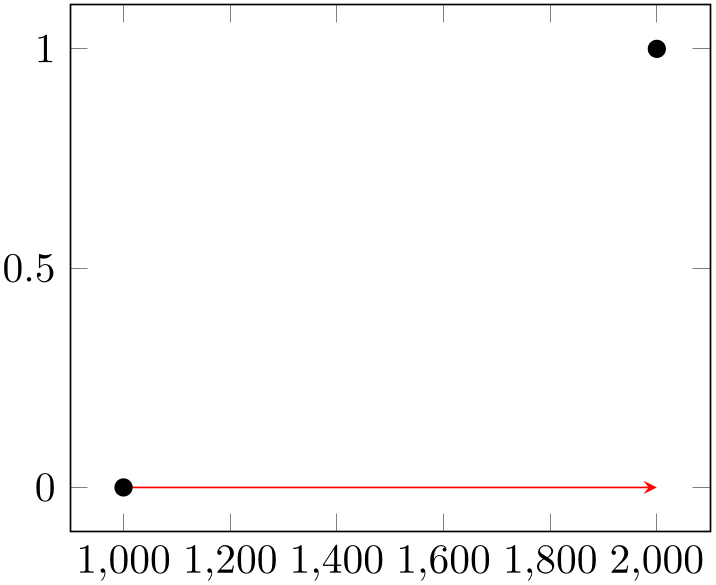
As noted in the documentation for axis cs, adding two coordinates by means of the TikZ ++ operator may have unexpected effects. The correct way for ++ operations is axis direction cs:

% Preamble: \pgfplotsset{width=7cm,compat=1.18}
\begin{tikzpicture}
\begin{axis}
\draw [red,-stealth]
(1000,0)
-- % = line-to
++ % = calculate a vector sum
(axis direction cs:1000,0);
\addplot [only marks,mark=*]
                            coordinates
                    { (1000,0) (2000,1) };
\end{axis}
\end{tikzpicture}
Here, the target of the red arrow is the position (2000,0) as expected.
Using relative positions is mainly useful for linear axes. Applying this command to log-axes might still work, but it requires more care.
One use case is to supply lengths – for example in order to support circle or ellipse paths. The
correct way to draw an ellipse in pgfplots would be to specify the two involved radii by means
of two (axis direction cs:x,y) expressions. In general, this is possible if you use the basic level macros \pgfpathellipse and
\pgfplotspointaxisdirectionxy. Please refer to the documentation of
\pgfplotspointaxisdirectionxy for two
examples of drawing arbitrary ellipses by means of this method.
Since drawing circles and ellipses inside of an axis is a common use case,
pgfplots automatically communicates its coordinate system transformations to TikZ:
whenever you write \draw ellipse[x radius=x,y radius=y], the arguments
x
and
y
are considered to be pgfplots direction vectors and are handed over to
axis direction cs. Consequently, ellipses with axis parallel radii are straightforward and use the normal TikZ syntax:
% Preamble: \pgfplotsset{width=7cm,compat=1.18}
% requires \pgfplotsset{compat=1.5.1} !
\begin{tikzpicture}
\begin{axis}[
xmin=-2.5, xmax=2.5,
ymin=-2.5, ymax=2.5,
xtick={-2,-1,0,1,2},
ytick={-2,-1,0,1,2},
grid=major,
]
% standard tikz syntax:
\draw [black] (0,0) ellipse [
x radius=1,
y radius=2,
];
\draw [red] (0,0) ellipse [
rotate=90,
x radius=1,
y radius=2,
];
% see \pgfplotspointaxisdirectionxy
% for arbitrary ellipses
\end{axis}
\end{tikzpicture}
Here, the two ellipses are specified as usual in TikZ. pgfplots ensures that all necessary transformations are applied to the two radii. Note that pgfplots usually has different axis scales for \(x\) and \(y\). As a consequence, the rotated red ellipse does not fit into the axis lines; we would need to use axis equal to allow properly rotated ellipses.
this modification to circles and ellipses requires \pgfplotsset{compat=1.5.1}.
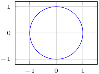
The same applies to circles: in the standard view, a circle with radius=\(r\) will appear as an ellipse due to the different axis scales. Supplying axis equal results in true circles:
% Preamble: \pgfplotsset{width=7cm,compat=1.18}
% requires \pgfplotsset{compat=1.5.1} !
\begin{tikzpicture}
\begin{axis}[tiny,enlargelimits,
xmin=-1,xmax=1,
ymin=-1,ymax=1,
xtick={-1,0,1},
ytick={-1,0,1},
grid=major,
]
\draw [blue] (0,0) circle [radius=1];
\end{axis}
\end{tikzpicture}

% Preamble: \pgfplotsset{width=7cm,compat=1.18}
\begin{tikzpicture}
\begin{axis}[tiny,enlargelimits,
axis equal,
xmin=-1,xmax=1,
ymin=-1,ymax=1,
xtick={-1,0,1},
ytick={-1,0,1},
grid=major,
]
\draw [blue] (0,0) circle [radius=1];
\end{axis}
\end{tikzpicture}
In case you need access to axis direction cs inside of math expressions, you can employ the additional math function transformdirectionx. It does the same as axis direction cs, but only in \(x\) direction. The result of transformdirectionx is a dimensionless unit which can be interpreted relative to the current pgf \(x\) unit vector \(e_x\) (see the documentation of \pgfplotstransformdirectionx for details). There are the math commands transformdirectionx, transformdirectiony, and (if the axis is three-dimensional) transformdirectionz. Each of them defines \pgfmathresult to contain the result of \pgfplotstransformdirectionx (or its variants for \(y\) and \(z\), respectively).
-
Coordinate system rel axis cs 
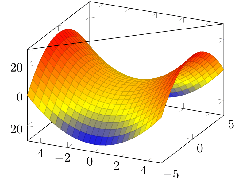
The “relative axis coordinate system”, rel axis cs, uses the complete axis vectors as units. That means ‘\(x=0\)’ denotes the point on the lower \(x\)-axis range and ‘\(x=1\)’ the point on the upper \(x\)-axis range (see the remark below for x dir=reverse).

% Preamble: \pgfplotsset{width=7cm,compat=1.18}
\begin{tikzpicture}
\begin{axis}
\addplot3 [surf] {x^2 - y^2};
\draw (rel axis cs:0,0,1)
-- (rel axis cs:1,1,1);
\end{axis}
\end{tikzpicture}
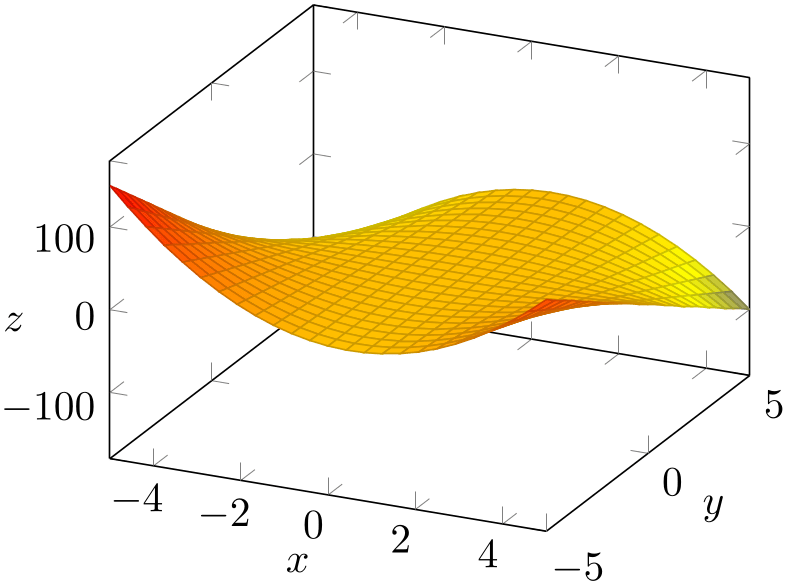
% Preamble: \pgfplotsset{width=7cm,compat=1.18}
\begin{tikzpicture}
\begin{axis}[
xlabel=$x$,
ylabel=$y$,
zlabel=$z$,
every axis x label/.style={
at={(rel axis cs:0.5,-0.15,-0.15)}},
every axis y label/.style={
at={(rel axis cs:1.15,0.5,-0.15)}},
every axis z label/.style={
at={(rel axis cs:-0.15,-0.15,0.5)}},
]
\addplot3 [surf] {x*(1-x)*y};
\end{axis}
\end{tikzpicture}
Points identified by rel axis cs use the syntax
(rel axis cs:x,y) or
(rel axis cs:x,y,z)
where
x,
y
and
z
are coordinates or constant mathematical expressions. The second syntax is only available in three dimensional axes.
There is one specialty: if you reverse an axis (with x dir=reverse), points provided by rel axis cs will be unaffected by the axis reversal. This is intended to provide consistent placement even for reversed axes. Use allow reversal of rel axis cs=false to disable this feature.
There is also a low-level interface to access the transformations and coordinates, see Chapter 9 on page (page for part 9).
-
Predefined node current plot begin 
This coordinate will be defined for every plot and can be used as
trailing path commands
or after a plot. It is the first coordinate of the current plot.
-
Predefined node current plot end 
This coordinate will be defined for every plot. It is the last coordinate of the current plot.
-
/pgfplots/allow reversal of rel axis cs=true|false (initially true) 
A fine-tuning key which specifies how to deal with x dir=reverse and rel axis cs and ticklabel cs.
The initial configuration true means that points placed with rel axis cs and/or ticklabel cs will be at the same position inside of the axes even if its ordering has been reversed. The choice false will disable the special treatment of x dir=reverse.
61 As of pgfplots version 1.11 and compat=1.11. All older versions explicitly require the prefix; coordinates without the prefix will be placed at the wrong position.
4.17.2Changing the Appearance of Individual Coordinates
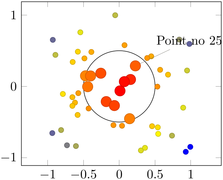
Some plot handlers, especially scatter plots in their different variants, support to modify the appearance of individual markers. To this end, they accept the syntax coordinate style:
% Preamble: \pgfplotsset{width=7cm,compat=1.18}
\begin{tikzpicture}
\begin{axis}[axis equal]
\addplot[
scatter,
only marks,
samples=50,
point meta=100-sqrt(x^2+y^2),
coordinate style/.condition=
{sqrt(x^2+y^2) < 0.5}{scale=2},
coordinate style/.condition={\coordindex == 25}{
/pgfplots/scatter/@post marker code/.add code={
\node [pin=45:Point no 25] {};
}{},
},
] (rand,rand);
\draw (0,0) circle (0.5);
\end{axis}
\end{tikzpicture}
The previous example is a scatter plot of random points. The first coordinate style ensures that all points falling into the circle of radius \(0.5\) are drawn twice as large. The second coordinate style applies special drawing instructions to the point with index \(25\): it attaches a pin.
The key coordinate style is documented on page (??).
4.17.3Placing Nodes on Coordinates of a Plot
The \addplot command is not only used for pgfplots, it can also carry additional drawing instructions which are handed over to TikZ after the plot’s path is complete. Among others, this can be used to add further nodes on the path.
-
/tikz/pos={
fraction}
The
fraction
identifies a part of the recently completed plot if it is used before the trailing semicolon:
Here, the [yshift=8pt] tells TikZ to shift all following nodes upwards. The node[pos=0] {$0$} instruction tells TikZ to add a text node at \(0\%\) of the recently completed plot. The relative position \(0\%\) (pos=0) refers to the first coordinate which has been seen by pgfplots, and \(100\%\) (pos=1) refers to the last coordinate. Any value between \(0\) and \(1\) is interpolated in-between. Note that all these nodes belong to the plot’s visualization (which is terminated by the semicolon). Consequently, all these nodes inherit the same graphic settings (like color choices).
The position on the plot is computed by pgfplots using logical coordinates. That means: it computes the overall length of the curve before the curve is projected to screen coordinates and identifies the desired position.62 Afterwards, it projects the final position to screen coordinates. Thus, the position identifies a location on the plot which is always the same, even in case of a rotated three-dimensional axis. pgfplots will linearly interpolate the fraction between successive coordinates.
Valid choices for
fraction
are any numbers in the range \([0,1]\).
Note that the precise meaning of pos depends on the current plot handler: for most plot handlers, it defaults to linear interpolation (as in the examples above). For only marks, scatter, ybar, xbar, ybar interval, and xbar interval, it snaps to the nearest encountered coordinate. In this context, “snap to nearest” means that pos=\(p\) refers to the coordinate with index \(i = \text {round}(p \cdot N)\) where \(N\) is the total number of points:
% Preamble: \pgfplotsset{width=7cm,compat=1.18}
\begin{tikzpicture}
\begin{axis}[title=Snap to nearest for scatter plots]
\addplot+ [only marks]
                            coordinates
                    { (0,0) (1,1) (2,2) (3,3) }
node [pos=0, pin=0 :0 ] {}
node [pos=0.1, pin=90 :0.1 ] {}
node [pos=0.2, pin=200:0.2 ] {}
node [pos=0.3, pin=135:0.3 ] {}
node [pos=0.4, pin=0 :0.4 ] {}
node [pos=0.5, pin=60 :0.5 ] {}
node [pos=0.75,pin=180:0.75] {}
node [pos=1, pin=90 :1 ] {}
;
\end{axis}
\end{tikzpicture}
the previous example shows that pos=\(p\) maps to one of the four available coordinates, namely the one whose index is closest to \(p\cdot N\). Note that in such a case, the distance between coordinates is irrelevant – only the coordinate index counts.
Note that the fact that pgfplots uses logical coordinates to compute the target positions can produce unexpected effects if \(x\) and \(y\) axis operate on a different scales. Suppose, for example, that \(x\) is always of order \(10^3\) whereas \(y\) is of order \(10^{-3}\). In such a scenario, the \(y\)-coordinate have no significant contribution to the curve’s length – although the rescaled axes clearly show “significant” \(y\) dynamics. Consider using axis equal together with pos to produce comparable effects.
-
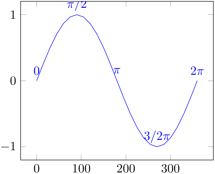
/tikz/sloped(initially false) 
Providing the TikZ key sloped to a node identified by pos causes it to be rotated such that it adapts to the plot’s gradient.
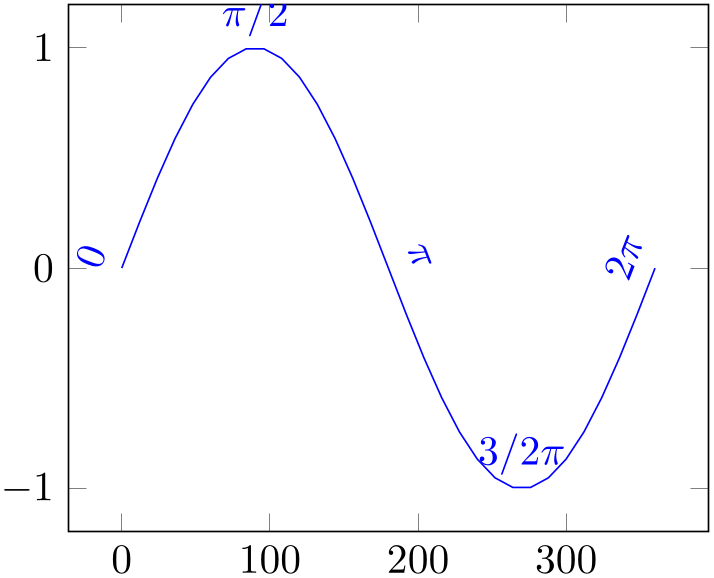
% Preamble: \pgfplotsset{width=7cm,compat=1.18}
\begin{tikzpicture}
\begin{axis}
\addplot [blue,domain=0:360,samples=31] {sin(x)}
[every node/.style={yshift=8pt},sloped]
node [pos=0] {$0$}
node [pos=0.25] {$\pi/2$}
node [pos=0.5] {$\pi$}
node [pos=0.75] {$3/2\pi$}
node [pos=1] {$2\pi$}
;
\end{axis}
\end{tikzpicture}
Note that the sequence in which sloped and shift transformations are applied is important: if shifts are applied first (as would be the case without the every node/.style construction), the shifts do not respect the rotation. If sloped is applied first, any subsequent shifts will be applied in the rotated coordinates. Thus, the case every node/.style={yshift=8pt} shifts every node by 8pt in direction of its normal vector.
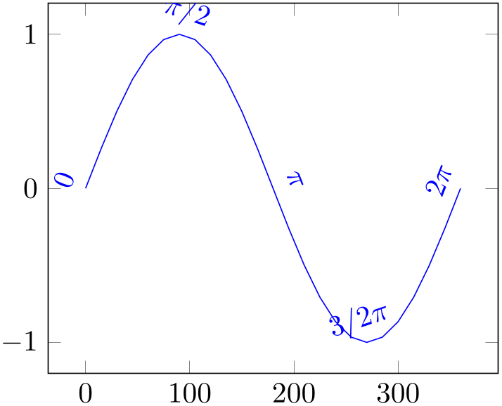
The sloped transformation is based on the gradient between two points (the two points adjacent to pos). Consequently, it inherits any sampling weaknesses. To see this, consider the example above with a different number of samples:

% Preamble: \pgfplotsset{width=7cm,compat=1.18}
% same as above with different number of samples
\begin{tikzpicture}
\begin{axis}
\addplot [blue,domain=0:360,samples=25] {sin(x)}
[every node/.style={yshift=8pt},sloped]
node [pos=0] {$0$}
node [pos=0.25] {$\pi/2$}
node [pos=0.5] {$\pi$}
node [pos=0.75] {$3/2\pi$}
node [pos=1] {$2\pi$}
;
\end{axis}
\end{tikzpicture}
Here, the two extreme points have small slopes due to the sampling. While this does not seriously affect the quality of the plot, it has a huge impact on the transformation matrices. Keep this in mind when you work with sloped (perhaps it even helps to add a further rotate argument).
-
/tikz/allow upside down=true|false (initially false) 
If /tikz/sloped is enabled and one has some difficult line plot, the transformation may cause nodes to be drawn upside down. The default configuration allow upside down=false will switch the rotation matrix, whereas allow upside down allows this case.
-
/tikz/pos segment={
segment index} (initially empty)
Occasionally, one has a single plot which consists of multiple segments (like those generated by empty line=jump or contour prepared). The individual segments will typically have different lengths, so it is tedious to identify a position on one of these segments.
If pos segment=segment index
is non-empty, the key pos=fraction
is interpreted relatively to the provided segment rather than the whole plot. The argument
segment index
is an integer, where \(0\) denotes the first segment.
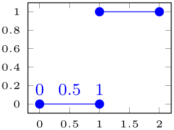
% Preamble: \pgfplotsset{width=7cm,compat=1.18}
\begin{tikzpicture}
\begin{axis}[tiny]
                        \addplot coordinates
                    {
(0,0) (1,0)
(1,1) (2,1)
}
[pos segment=0,yshift=7pt,font=\footnotesize]
node [pos=0] {0}
node [pos=0.5] {0.5}
node [pos=1] {1};
\end{axis}
\end{tikzpicture}
Here, the plot has two segments. However, all three annotation nodes are placed with pos segment=0.

% Preamble: \pgfplotsset{width=7cm,compat=1.18}
\begin{tikzpicture}
\begin{axis}
\addplot3 [contour lua,domain=0:1] {x*y}
[sloped,
allow upside down,
pos segment=2,
every node/.style={yshift=7pt},
]
node [pos=0] {0}
node [pos=0.5] {0.5}
node [pos=1] {1}
;
\end{axis}
\end{tikzpicture}
This plot has four segments (which are generated automatically by the plot handler). The annotation nodes are placed on the third segment, where sloped causes them to be rotated, allow upside down improves the rendering of the ‘\(0\)’, and every node/.style install a shift in direction of the normal vector (see the documentation of sloped for details).
Occasionally, one wants to place a node using pos and one wants to typeset the coordinates of that point inside of the node. This can be accomplished using \pgfplotspointplotattime:
-
\pgfplotspointplotattime 
-
\pgfplotspointplotattime{
fraction}
-
/data point/x(no value) 
-
/data point/y(no value) 
-
/data point/z(no value) 
This command is part of the pos={fraction} implementation: it defines the current point of pgf to
fraction
of the current plot. Without an argument in curly braces,
\pgfplotspointplotattime will take the
current argument of the pos key.
Thus, the command computes the basic pgf coordinates – but it also returns the logical coordinates of the resulting point into the following keys:
After \pgfplotspointplotattime returns, these macros contain the \(x\)-, \(y\)-, and \(z\)-coordinates of the resulting point. They can be used by means of \pgfkeysvalueof{/data point/x}, for example.
% Preamble: \pgfplotsset{width=7cm,compat=1.18}
\begin{tikzpicture}
\begin{axis}
\addplot {x}
[left,/pgf/number format/relative=0]
node [pos=0.5] {
\pgfplotspointplotattime
$(\pgfmathprintnumber
{\pgfkeysvalueof{/data point/x}},
\pgfmathprintnumber
{\pgfkeysvalueof{/data point/y}})$
}
node [pos=0.25] {
\pgfplotspointplotattime
$(\pgfmathprintnumber
{\pgfkeysvalueof{/data point/x}},
\pgfmathprintnumber
{\pgfkeysvalueof{/data point/y}})$
}
node [pos=0.7,pin=180:{
\pgfplotspointplotattime{0.7}
$(\pgfmathprintnumber
{\pgfkeysvalueof{/data point/x}},
\pgfmathprintnumber
{\pgfkeysvalueof{/data point/y}})$
}] {}
;
\end{axis}
\end{tikzpicture}
In the example above, three nodes have been placed using different pos= arguments. Invoking \pgfplotspointplotattime inside of the associated node’s body checks if pos already has a value and uses that value. The third node displays the coordinates inside of a pin. Due to internals of TikZ, the pin knows nothing about the pos=0.7 argument of its enclosing node, so we need to replicate the ‘0.7’ argument for \pgfplotspointplotattime{0.7}. The /pgf/number format/relative=0 style causes the number printer to round relative to \(10^0\) (compare against the same example without this style).
In case you have symbolic x coords (or any other x coord inv tafo which produces non-numeric results), the output stored in /data point/x will be the symbolic expression:

% Preamble: \pgfplotsset{width=7cm,compat=1.18}
\begin{tikzpicture}
\begin{axis}[symbolic x coords={A,B,C,D}]
                            \addplot coordinates
                        {(A,0) (B,1) (C,1) (D,2)}
[left]
node [pos=0.3] {
\pgfplotspointplotattime
                                        $(\pgfkeysvalueof{/data
                        point/x},
\pgfmathprintnumber
{\pgfkeysvalueof{/data point/y}})$
}
node [pos=0.7,pin=180:{
\pgfplotspointplotattime{0.7}
                                        $(\pgfkeysvalueof{/data
                        point/x},
\pgfmathprintnumber
{\pgfkeysvalueof{/data point/y}})$
}] {}
;
\end{axis}
\end{tikzpicture}
In that specific case, you have to avoid \pgfmathprintnumber since the argument is no number. Note that symbolic x coords cannot return fractions between, say, \(A\) and \(B\) as you would expect. However, the point will still be placed at the fractional position (unless you have a scatter or bar plot).
The computation of coordinates for the pos feature is computationally expensive for plots with many points. To reduce time, pgfplots will cache computed values: invoking the command \pgfplotspointplotattime multiple times with the same argument will reuse the computed value.
62 This can be a time-consuming process. Consider using the external library if you have lots of such figures.
4.17.4Placing Decorations on Top of a Plot
TikZ comes with the powerful decorations library (or better: set of libraries). Decorations allow to replace or extend an existing path by means of fancy additional graphics. An introduction into the decorations functionality of TikZ is beyond the scope of this manual and the interested reader should read the associated section in [7].
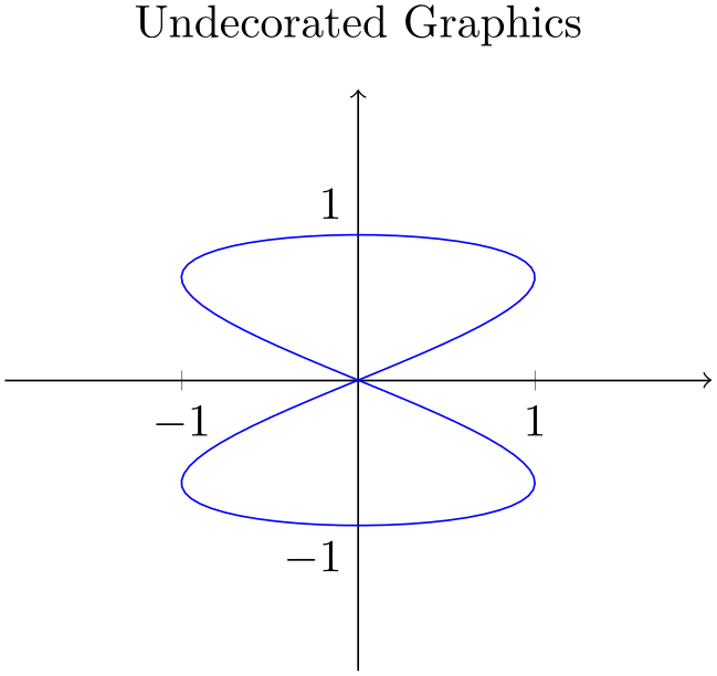
This section shows how to use decorations to enhance plots in pgfplots. Suppose you have some graphics for which you would like to add “direction pointers”:

% Preamble: \pgfplotsset{width=7cm,compat=1.18}
\begin{tikzpicture}[]
% An undecorated graphics with a lot of
% pretty-printing styles:
\begin{axis}[
axis lines=middle,
title=Undecorated Graphics,
xmin=-2, xmax=2, ymin=-2, ymax=2,
xtick={-1,1}, ytick={-1,1},
% this disables the standard
% tick label *text* (but not the line)
yticklabel=\ ,
extra description/.code={
% this generates custom y labels to implement
% individual styles for every tick:
                        \node [below
                left] at (axis cs:0,-1) {$-1$};
                        \node [above
                left] at (axis cs:0,1) {$1$};
},
axis line style={->},
]
\addplot [blue,samples=100,domain=0:2*pi]
({sin(deg(2*x))}, {sin(deg(x))});
\end{axis}
\end{tikzpicture}
Our aim is to add short pointers indicating the direction of the parametrization.
The solution is to use \usetikzlibrary{decorations.markings} and a decoration inside of \addplot:
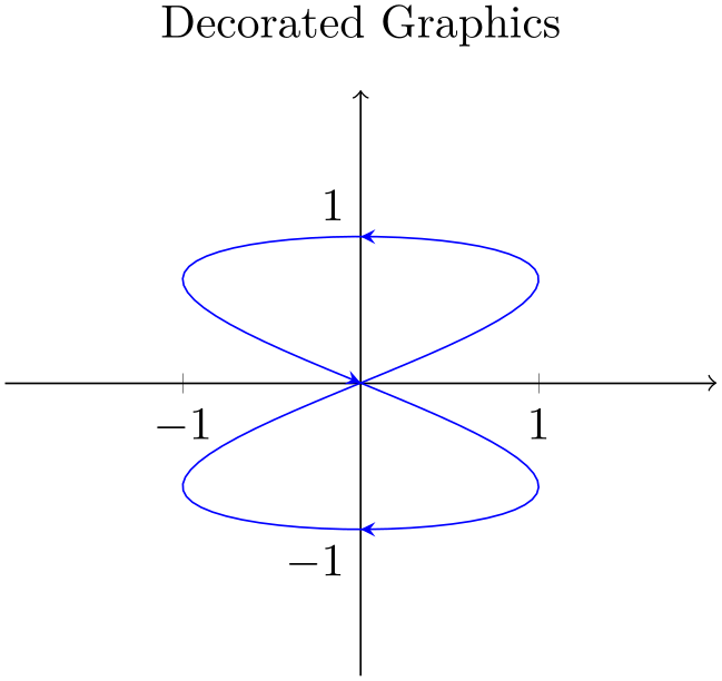
% Preamble: \pgfplotsset{width=7cm,compat=1.18}
% requires \usetikzlibrary{decorations.markings}
\begin{tikzpicture}[]
% Same as in previous example, but with decorations:
\begin{axis}[
axis lines=middle,
title=Decorated Graphics,
xmin=-2, xmax=2, ymin=-2, ymax=2,
xtick={-1,1}, ytick={-1,1},
% this disables the standard
% tick label *text* (but not the line)
yticklabel=\ ,
extra description/.code={
% this generates custom y labels to implement
% individual styles for every tick:
                        \node [below
                left] at (axis cs:0,-1) {$-1$};
                        \node [above
                left] at (axis cs:0,1) {$1$};
},
axis line style={->},
]
\addplot[blue,samples=100,domain=0:2*pi,
postaction={decorate},% ------
                      decoration={markings, %
                ------
mark=at position 0.25 with {\arrow{stealth}},
mark=at position 0.5 with {\arrow{stealth}},
mark=at position 0.75 with {\arrow{stealth}}}
] ({sin(deg(2*x))}, {sin(deg(x))});
\end{axis}
\end{tikzpicture}
The only changes are in the option list for \addplot: it contains a postaction={decorate} which activates the decoration (without replacing the original path) and some specification decoration containing details about how to decorate the path.
A discussion of details of the decorations libraries is beyond the scope of this manual (see [7] for details), but the main point is to add the required decorations to \addplot and its option list.