Manual for Package pgfplots
2D/3D Plots in LATeX, Version 1.18.2
https://github.com/pgf-tikz/pgfplots
The Reference
4.12Error Bars
An error bar is used to indicate the reliability of a data point. Typically, a data point is just \((x,y)\). The reliability would be indicated by additional values, i.e. by means of an error bound \(\epsilon _x\) which characterizes the difference between the coordinate \(x\) provided in the plot data and the precise value \(\tilde x\) (which is unknown). The reliability can be indicated for both \(x\) and \(y\) independently (although \(y\) might be the typical candidate). Error bounds can be expressed as absolute errors, i.e. of the form
\(\seteqnumber{0}{}{0}\)\begin{equation*} \lvert {x-\tilde x}\rvert \le \epsilon _x, \quad \lvert {y-\tilde y}\rvert \le \epsilon _y \end{equation*}
where \(\tilde x\) and \(\tilde y\) are the (unknown) precise values and \(x\) and \(y\) are the actual values of the plot. However, they can also be provided relative to the input values, i.e. of the form
\(\seteqnumber{0}{}{0}\)\begin{equation*} \frac {\lvert {x-\tilde x}\rvert } {\lvert \tilde x\rvert } \le \epsilon _x, \quad \frac {\lvert {y-\tilde y}\rvert } {\lvert \tilde y\rvert } \le \epsilon _y. \end{equation*}
A relative error of \(10\%\) would result in an error value of \(0.1\) (relative to the precise quantity \(\tilde y\)). Clearly, relative errors are only useful if the precise value if not zero, i.e. \(\tilde x, \tilde y \neq 0\).
pgfplots allows to provide the “error values” for each coordinate independently. Thus, it may find some value \(\epsilon _x\) and/or \(\epsilon _y\). Depending on the configuration, it interprets the encountered value as absolute or relative error. The error value can be the same for every coordinate, for example if you know that each \(y\)-coordinate has a fixed error of \(10\%\). The error value can also be different for every coordinate in which it is said to be “explicitly provided”. In fact, pgfplots also features asymmetric error values, i.e. the lower bound on the error can be different from the upper bound. Thus, a two-dimensional data point \((x,y)\) can have up to four distinct error values which have to be provided by the end-user.
Thus, the end-user has to provide all needed error values and a configuration to express if these values are to be interpreted as relative or absolute error and if the values are to be expected explicitly for every data point or if they are fixed.
% Preamble: \pgfplotsset{width=7cm,compat=1.18}
\begin{tikzpicture}
\begin{axis}
\addplot+ [
error bars/.cd,
y dir=plus,y explicit,
] coordinates {
                        (0,0)     +-
                (0.5,0.1)
                        (0.1,0.1) +-
                (0.05,0.2)
(0.2,0.2) +- (0,0.05)
(0.5,0.5) +- (0.1,0.2)
                        (1,1)     +-
                (0.3,0.1)
};
\end{axis}
\end{tikzpicture}
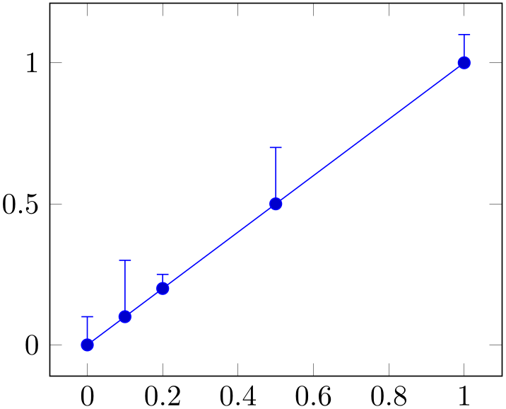
The preceding example has two keys: y dir=plus configures pgfplots to activate error bars for \(y\)-coordinates, but only upper bounds. The key y explicit tells pgfplots to expect absolute values in the input data stream. In our case above, the input data stream is an \addplot coordinates which uses the special error value syntax +- \((\epsilon _x, \epsilon _y)\), see the Section 4.12.1.1 for details.
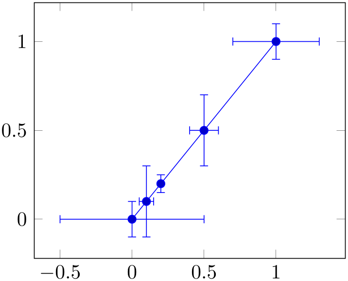
It is allowed if the input data contains more error values than needed: our example above has error values for both \(x\) and \(y\) and it also contains lower bounds (since +- defines upper- and lower bounds simultaneously).
Consequently, the remaining values can be visualized as well:
% Preamble: \pgfplotsset{width=7cm,compat=1.18}
\begin{tikzpicture}
\begin{axis}
\addplot+ [
error bars/.cd,
y dir=both,y explicit,
x dir=both,x explicit,
] coordinates {
                        (0,0)     +-
                (0.5,0.1)
                        (0.1,0.1) +-
                (0.05,0.2)
(0.2,0.2) +- (0,0.05)
(0.5,0.5) +- (0.1,0.2)
                        (1,1)     +-
                (0.3,0.1)
};
\end{axis}
\end{tikzpicture}
Error bars inherit all drawing options of the associated plot, but they use their own error mark and additional style arguments.
-
/pgfplots/error bars/x dir=none|plus|minus|both (initially none) 
-
/pgfplots/error bars/y dir=none|plus|minus|both (initially none) 
-
/pgfplots/error bars/z dir=none|plus|minus|both (initially none) 
The initial configuration none draws no error bars at all in the provided direction.
The configuration plus draws only upper bounds in the direction of interest.
The configuration minus draws only lower bounds in the direction of interest.
The configuration both draws upper and lower bounds in the direction of interest.
In every case, the actual error value and its character (absolute or relative) is to be determined by other options (see below). If, for some reason, the error value is missing, the error bar is omitted.
-
/pgfplots/error bars/x fixed={
 value
value } (initially 0)
-
/pgfplots/error bars/y fixed={
 value
value } (initially 0)
-
/pgfplots/error bars/z fixed={
 value
value } (initially 0)
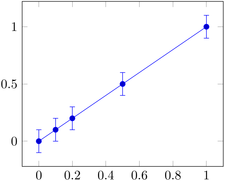
Provides a common, absolute error \(\epsilon _x=\text {\meta {value}}\) for all input coordinates.
% Preamble: \pgfplotsset{width=7cm,compat=1.18}
\begin{tikzpicture}
\begin{axis}
\addplot+ [
error bars/.cd,
y dir=both,y fixed=0.1,
] coordinates {
(0,0)
(0.1,0.1)
(0.2,0.2)
(0.5,0.5)
(1,1)
};
\end{axis}
\end{tikzpicture}
For linear \(x\)-axes, the error mark is drawn at \(x \pm \epsilon _x\) while for logarithmic \(x\)-axes, it is drawn at \(\log ( x \pm \pgfplotserror x)\).
-
/pgfplots/error bars/x fixed relative={
 percent
 } (initially 0)
-
/pgfplots/error bars/y fixed relative={
 percent
 } (initially 0)
-
/pgfplots/error bars/z fixed relative={
 percent
 } (initially 0)
Provides a common,
relative error \(\epsilon _x = \text {\meta {percent}} \cdot x\) for all input coordinates. The argument
 percent
 is thus given relatively to input \(x\)-coordinates such that \(\text {\meta {percent}} = 1\) means \(100\%\).
Error marks are thus placed at \(x \cdot (1 \pm \epsilon _x)\) for linear axes and at \(\log (x \cdot (1 \pm \epsilon _x))\) for logarithmic axes. Computations are performed in floating point for linear axis and using the identity \(\log (x \cdot (1 \pm \epsilon _x)) = \log (x) + \log ( 1 \pm \epsilon _x)\) for logarithmic scales.
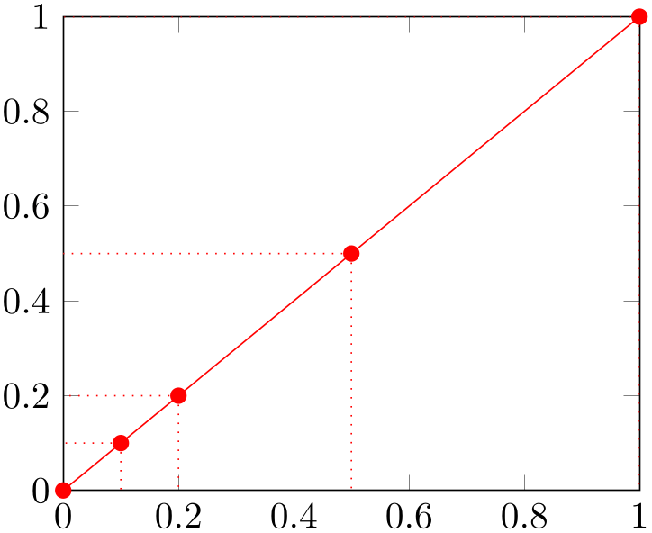
The following example shows that fixed error values \(\epsilon _x\) are independent of the input values.
% Preamble: \pgfplotsset{width=7cm,compat=1.18}
\begin{tikzpicture}
\begin{axis}[enlargelimits=false]
\addplot [red,mark=*] plot [
error bars/.cd,
y dir=minus,y fixed relative=1,
x dir=minus,x fixed relative=1,
error mark=none,
error bar style={dotted},
] coordinates {
(0,0) (0.1,0.1) (0.2,0.2)
(0.5,0.5) (1,1)
};
\end{axis}
\end{tikzpicture}
-
/pgfplots/error bars/x explicit(no value) 
-
/pgfplots/error bars/y explicit(no value) 
-
/pgfplots/error bars/z explicit(no value) 
Configures the error bar algorithm to draw \(x\)-error bars at any input coordinate for which user-specified errors are available. Each error is interpreted as absolute error, see x fixed for details.
The different input formats of errors are described in Section 4.12.1.
-
/pgfplots/error bars/x explicit relative(no value) 
-
/pgfplots/error bars/y explicit relative(no value) 
-
/pgfplots/error bars/z explicit relative(no value) 
Configures the error bar algorithm to draw \(x\)-error bars at any input coordinate for which user-specified errors are available. Each error is interpreted as relative error, that means error marks are placed at \(x (1 \pm \text {\meta {value}}(x))\) (works as for error bars/x fixed relative).
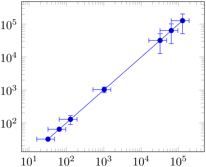
% Preamble: \pgfplotsset{width=7cm,compat=1.18}
\begin{tikzpicture}
\begin{loglogaxis}
\addplot+ [
error bars/.cd,
x dir=both,x fixed relative=0.5,
y dir=both,y explicit relative,
] table [x=x,y=y,y error=error] {
                            x
                          y
                          error
                            32      32
                         0
                            64      64
                         0
                            128     128
                        0.3
1024 1024 0.2
32068 32068 0.6
64000 64000 0.6
128000 128000 0.6
};
\end{loglogaxis}
\end{tikzpicture}
-
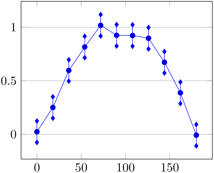
/pgfplots/error bars/error mark=
 marker
 (initially -)
Sets an error marker for
any error bar.
 marker
 is expected to be a valid plot mark, see Section 4.7.
% Preamble: \pgfplotsset{width=7cm,compat=1.18}
\begin{tikzpicture}
\pgfmathsetseed{42}
\begin{axis}[
ymajorgrids,
]
\addplot+ [
domain=0:180,
samples=11,
error bars/.cd,
y dir=both, y fixed=0.1,
error mark=diamond*,
] {sin(x) + rand*0.1};
\end{axis}
\end{tikzpicture}
-
/pgfplots/error bars/error mark options={
 key-value-list
 } (initially rotate=90)
Sets a key–value list of options for any error mark. This option works similarly to the TikZ ‘mark options’ key.
-
/pgfplots/error bars/error bar style={
 key-value-list
 }
}
Appends the argument to ‘/pgfplots/every error bar’ which is installed at the beginning of every error bar.
-
/pgfplots/error bars/draw error bar/.code 2 args={
 ...
... }
}
-
• the source point, \((x,y)\) and
-
• the target point, \((\tilde x,\tilde y)\).
Allows to change the default drawing commands for error bars. The two arguments are
Both are determined by pgfplots according to the options described above. The default code is
\pgfplotsset{
/pgfplots/error bars/draw error bar/.code 2 args={
\pgfkeysgetvalue{/pgfplots/error bars/error mark}
{\pgfplotserrorbarsmark}
\pgfkeysgetvalue{/pgfplots/error bars/error mark options}
{\pgfplotserrorbarsmarkopts}
                            \draw #1
                    -- #2 node [pos=1,sloped,allow upside down] {
\expandafter\tikz\expandafter[\pgfplotserrorbarsmarkopts]{
\expandafter\pgfuseplotmark\expandafter{\pgfplotserrorbarsmark}
\pgfusepath{stroke}}
};
},
}
4.12.1Input Formats of Error Coordinates
Error bars with explicit error estimations for single data points require some sort of input format. This applies to error bars/x explicit and error bars/x explicit relative.
4.12.1.1Error Coordinates and Coordinate Lists
Error bar coordinates can be read from ‘\addplot coordinates’ in which they are expected after data point as such:
where \((1,2) \pm (0.4,0.2)\) is the first coordinate, \((2,4) \pm (1,0)\) the second and so forth. The point \((3,5)\) has no error coordinate. The syntax +- defines symmetric error values, i.e. both upper and lower bound receive the same value.
Alternatively, one can use one of -= and += to define asymmetric values:

% Preamble: \pgfplotsset{width=7cm,compat=1.18}
\begin{tikzpicture}
\begin{axis}
\addplot+ [
error bars/.cd,
x dir=both, x explicit,
y dir=both, y explicit,
] coordinates {
(1.1,0.9) +=
(0.4,0.2) -= (0.1,0.1)
(2.7,2) -=
(1,0)
(3,3)
(3.8,4.2) +- (0.3,0.2)
};
\end{axis}
\end{tikzpicture}
If multiple items (like multiple +=) for one coordinate are specified, the last one takes precedence.
Keep in mind that these error values are only displayed as error bars if x dir and y dir are set appropriately.
The input type \addplot coordinates also allows point meta=explicit, i.e. values of the form
                \addplot coordinates
{(0,0) [4]};
This can be combined with error values. However, the point meta value in square brackets needs to be the last item:
                \addplot coordinates
                {(0,0) +- (0.1,0.2) [4]};
4.12.1.2Error Coordinates and Table Input
The ‘\addplot table’ format is
-
/pgfplots/table/x error={
 column name
 }
}
-
/pgfplots/table/y error={
 column name
 }
}
-
/pgfplots/table/z error={
 column name
 }
}
-
/pgfplots/table/x error index={
 column index
 }
}
-
/pgfplots/table/y error index={
 column index
 }
}
-
/pgfplots/table/z error index={
 column index
 }
}
-
/pgfplots/table/x error expr={
 math expression
 }
}
-
/pgfplots/table/y error expr={
 math expression
 }
}
-
/pgfplots/table/z error expr={
 math expression
 }
}
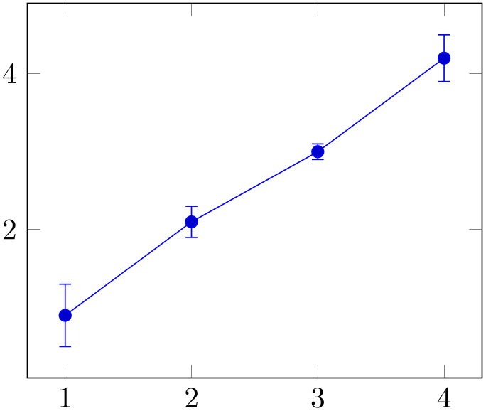
These keys define input sources for error bars with explicit error values.
The x error method provides an input column name (or
alias), the x error index method provides
input column indices and
x error expr works just as
table/x expr: it allows arbitrary mathematical expressions which may depend on any number of table columns using
\thisrow{ col name
 }.
}.
% Preamble: \pgfplotsset{width=7cm,compat=1.18}
\begin{tikzpicture}
\begin{axis}
\addplot+ [
error bars/.cd,
x dir=both, x explicit,
y dir=both, y explicit,
] table [y error=error] {
                            x   y
                      error
1 0.9 0.4
2 2.1 0.2
3 3 0.1
4 4.2 0.3
};
\end{axis}
\end{tikzpicture}
In addition, one can provide column indices using
\addplot table[x error index=COLINDEX,y error index=COLINDEX]
These options are used like the ‘x’ and ‘x index’ options.
If you need to specify math expressions, you can use x error expr:
\addplot table[x error expr=\thisrow{errorx}^2]
This is similar to x expr.
-
/pgfplots/table/x error plus={
 column name
 }
}
-
/pgfplots/table/y error plus={
 column name
 }
}
-
/pgfplots/table/z error plus={
 column name
 }
}
-
/pgfplots/table/x error plus index={
 column index
 }
}
-
/pgfplots/table/y error plus index={
 column index
 }
}
-
/pgfplots/table/z error plus index={
 column index
 }
}
-
/pgfplots/table/x error plus expr={
 math expression
 }
}
-
/pgfplots/table/y error plus expr={
 math expression
 }
}
-
/pgfplots/table/z error plus expr={
 math expression
 }
}
-
/pgfplots/table/x error minus={
 column name
 }
}
-
/pgfplots/table/y error minus={
 column name
 }
}
-
/pgfplots/table/z error minus={
 column name
 }
}
-
/pgfplots/table/x error minus index={
 column index
 }
}
-
/pgfplots/table/y error minus index={
 column index
 }
}
-
/pgfplots/table/z error minus index={
 column index
 }
}
-
/pgfplots/table/x error minus expr={
 math expression
 }
}
-
/pgfplots/table/y error minus expr={
 math expression
 }
}
-
/pgfplots/table/z error minus expr={
 math expression
 }
}
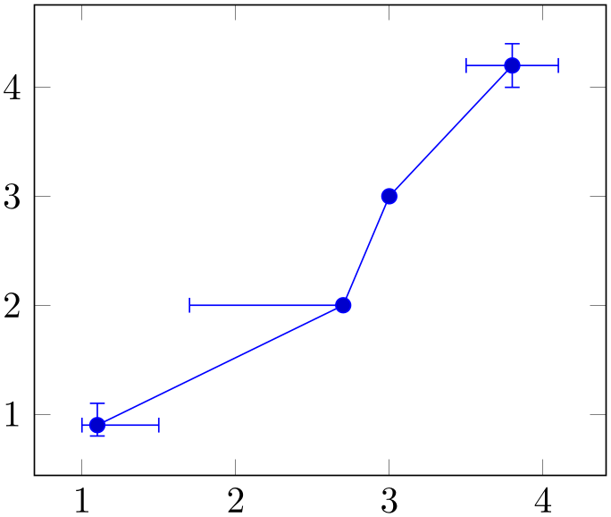
These keys define input sources for error bars with asymmetric error values, i.e. different values for upper and lower bounds.
They are to be used in the same way as x error. In fact, x error is just a style which sets both x error plus and x error minus to the same value.
% Preamble: \pgfplotsset{width=7cm,compat=1.18}
\begin{tikzpicture}
\begin{axis}
\addplot+ [
error bars/.cd,
x dir=both, x explicit,
y dir=both, y explicit,
] table [
x error plus=ex+,
x error minus=ex-,
y error plus=ey+,
y error minus=ey-,
] {
                            x   y
                      ex+  ey+  ex-  ey-
1.1 0.9 0.4 0.2 0.1 0.1
                            2.7 2   0    0
                       1    0
                            3   3   0    0
                       0    0
3.8 4.2 0.3 0.2 0.3 0.2
};
\end{axis}
\end{tikzpicture}