Manual for Package pgfplots
2D/3D Plots in LATeX, Version 1.18.2
https://github.com/pgf-tikz/pgfplots
The Reference
4.26TikZ Interoperability
pgfplots uses TikZ/pgf as its “backend layer”. This implies that it inherits most of TikZ’s graphical features and adds a lot of own stuff on top of it. However, the coordinate systems of TikZ and pgfplots do not match up – for good reason: pgfplots operates on logical (data) coordinates whereas TikZ operates on image coordinates.
Occasionally, one may want to synchronize both in order to generate a graphic. In this context, “synchronize both” means that they really use the same coordinate systems. This is far beyond the simple use case of “enrich a pgfplots picture by means of TikZ annotations”, compare Section 4.17.
Consequently, this section addresses the question how to match the coordinates from TikZ to pgfplots and vice versa. It explains how to match coordinates and it discusses the necessary configuration.
There are a couple of keys in pgfplots which control the mapping of coordinates. The purpose of these keys is to implement visualization techniques, but they do things different than TikZ (and they should). To match coordinates with TikZ, one needs the following aspects:
-
1. Restrict your visualization type: a logarithmic axis simply may not fit into TikZ (to be more precise: it may fit, but a TikZ unit will correspond to a log unit in pgfplots).
-
2. Configure matching unit vectors by means of the x and y keys. The default configuration of TikZ is to use x=1cm,y=1cm,z={(0,0)}. Note that these settings are usually overridden by pgfplots in order to respect width and height (and view for three-dimensional axes).
-
3. Disable the data scaling by means of disabledatascaling: pgfplots will internally apply linear coordinate transformations in order to provide the data range required for floating point arithmetics (using approximately floating point precision). Disabling the data scaling means to restrict yourself to the (small) data range supported by TikZ – but that’s probably what you want in that case.
-
4. Define anchor and position of the axis, probably using anchor=origin,at={(0,0)}. The at={(0,0)} configures pgfplots to place the axis at the TikZ position (0,0) whereas anchor=origin means that pgfplots will place its data origin \((0,0,0)\) at the place designated by at (see Section 4.19 for details).
-
5. Make sure that the pgfplots axis contains the data origin \((0,0,0)\) in the displayed data range (i.e. configure xmin, xmax, ymin, and ymax appropriately).
Without this, the anchor=origin key required in the previous item will be truncated to the next coordinate which is part of the displayed range.
Here is a simple example, first with TikZ:

\begin{tikzpicture}
\coordinate (Point) at (1,2);
\draw [gray] (-1,-1) grid (3,3);
\draw [blue,fill] (Point) circle (2pt)
node [right] {(1,2)}
;
\end{tikzpicture}
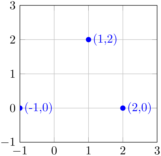
it displays a grid with \(x,y\in [-1,3]\) and shows a node inside of it. Now, we apply the keys discussed above to match this setting in pgfplots:

% Preamble: \pgfplotsset{width=7cm,compat=1.18}
\begin{tikzpicture}
\coordinate (Point) at (1,2);
\begin{axis}[
% tell pgfplots to "grab" the axis at its
% internal (0,0) coord:
anchor=origin,
% tell pgfplots to place its anchor at (0,0):
% (This is actually the default and can
% be omitted)
at={(0pt,0pt)},
% tell pgfplots to use the "natural" dimensions:
disabledatascaling,
% tell pgfplots to use the same unit vectors
% as tikz:
x=1cm,y=1cm,
%
% this is just as usual in pgfplots. I guess
% it is only useful if (0,0) is part of the
% range... try it out.
xmin=-1,xmax=3, ymin=-1,ymax=3,grid=both,
]
% this uses the point defined OUTSIDE of the axis
\draw [blue,fill] (Point) circle (2pt)
node [right] {(1,2)};
% this uses a TIKZ coordinate (2,0) in the axis:
\draw [blue,fill] (2,0) circle (2pt)
node [right] {(2,0)};
% this here will always work inside of an axis:
\draw [blue,fill] (-1,0) circle (2pt)
node [right] {(-1,0)};
\end{axis}
\end{tikzpicture}
The example demonstrates several things: first, it defines a coordinate in the enclosing tikzpicture and uses it inside of the axis (at the correct position). Second, it uses the standard TikZ coordinate (2,0) inside of the axis, and it is placed at the expected position. Third, it uses the approach provided by pgfplots by using the axis cs to designate a coordinate (this last approach does also work without the coordinate matching).
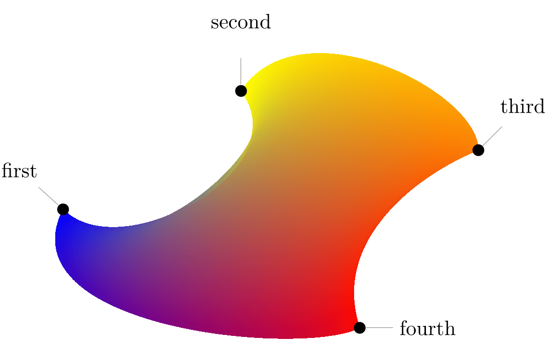
Here is an example which inserts a pgfplots graphics correctly into a tikzpicture:

% Preamble: \pgfplotsset{width=7cm,compat=1.18}
% requires \usepgfplotslibrary{patchplots}
\begin{tikzpicture}
\begin{axis}[
% tell pgfplots to "grab" the axis at its internal (0,0) coord:
anchor=origin,
% tell pgfplots to place its anchor at (0,0):
% (This is actually the default and can be omitted)
at={(0pt,0pt)},
% tell pgfplots to use the "natural" dimensions:
disabledatascaling,
% tell pgfplots to use the same unit vectors as tikz:
x=1cm,y=1cm,
%
hide axis,
]
\addplot [patch,patch type=coons,
shader=interp,point meta=explicit]
coordinates {
                            (0,0)      [0] %
                first corner
                            (1,-1)     [0] %
                bezier control point between (0) and (3)
                            (4,0.7)    [0] %
                bezier control point between (0) and (3)
%
                            (3,2)      [1] %
                second corner
                            (4,3.5)    [1] %
                bezier control point between (3) and (6)
                            (7,2)      [1] %
                bezier control point between (3) and (6)
%
                            (7,1)      [2] %
                third corner
                            (6,0.6)    [2] %
                bezier control point between (6) and (9)
                            (4.5,-0.5) [2] % bezier
                control point between (6) and (9)
%
                            (5,-2)     [3] %
                fourth corner
                            (4,-2.5)   [3] %
                bezier control point between (9) and (0)
                            (-1,-2)    [3] %
                bezier control point between (9) and (0)
};
\end{axis}
% this requires pgf 2.10
\begin{scope}[every node/.style={circle,inner sep=2pt,fill=black}]
\node [pin=140:first] at (0,0) {};
\node [pin=second] at (3,2) {};
\node [pin=45:third] at (7,1) {};
\node [pin=0:fourth] at (5,-2) {};
\end{scope}
\end{tikzpicture}
The example employs one of the patch plots of the patchplots library. Since these graphical elements typically require depth information (z buffering) and color data (point meta), they are only available inside of pgfplots. However, the configuration above ensures that coordinates match one-to-one between pgfplots and TikZ. The hide axis flag disables anything of pgfplots, so only the visualized patch plot remains.78