Manual for Package pgfplots
2D/3D Plots in LATeX, Version 1.18.2
https://github.com/pgf-tikz/pgfplots
The Reference
4.14Specifying the Plotted Range
4.14.1Configuration of Limits Ranges
-
/pgfplots/xmin={
 coord
coord }
}
-
/pgfplots/ymin={
coord}
-
/pgfplots/zmin={
coord}
-
/pgfplots/xmax={
coord}
-
/pgfplots/ymax={
coord}
-
/pgfplots/zmax={
coord}
-
/pgfplots/min={
coord}
-
/pgfplots/max={
coord}
These options allow to define the axis limits, i.e. the lower left and the upper right corner. Everything outside of the axis limits will be clipped away.
these values (and other related keys in this section) merely affect how pgfplots determines the axis’ range. The values are unrelated to function sampling. Please refer to domain in order to define the sampling range for plot expressions. It is valid to sample a larger or smaller range than the displayed portion of the axis. Use xmin and its friends to specify which portion of the axis is to be displayed.
Each of these keys is optional, and missing limits will be determined automatically from input data. Here, the
min and
max keys set limits for \(x\), \(y\) and \(z\) to the same
coord.
If \(x\) limits have been specified explicitly and \(y\) limits are computed automatically, the automatic computation of \(y\) limits will only considers points which fall into the specified \(x\)-range (and vice versa). The same holds true if, for example, only xmin has been provided explicitly: in that case, xmax will be updated only for points for which \(x \ge \;\)xmin holds. This feature can be disabled using clip limits=false.
Axis limits can be increased automatically using the enlargelimits option.
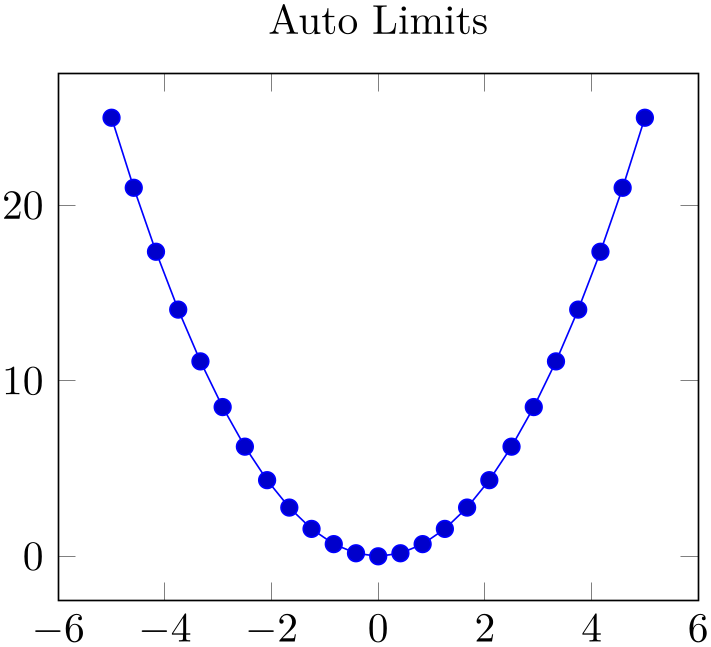
% Preamble: \pgfplotsset{width=7cm,compat=1.18}
\begin{tikzpicture}
\begin{axis}[
title=Auto Limits,
]
\addplot {x^2};
\end{axis}
\end{tikzpicture}
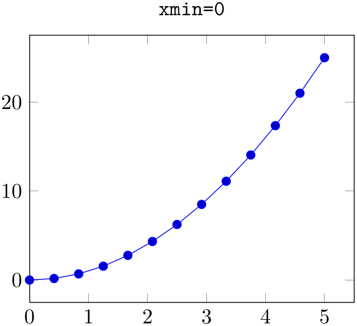
% Preamble: \pgfplotsset{width=7cm,compat=1.18}
\begin{tikzpicture}
\begin{axis}[
title={\texttt{xmin=0}},
xmin=0,
]
\addplot {x^2};
\end{axis}
\end{tikzpicture}
% Preamble: \pgfplotsset{width=7cm,compat=1.18}
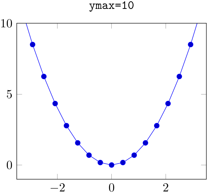
\begin{tikzpicture}
\begin{axis}[
title={\texttt{ymax=10}},
ymax=10,
]
\addplot {x^2};
\end{axis}
\end{tikzpicture}
Note that even if you provide ymax=10, data points with \(y>10\) will still be visualized – producing a line which leaves the plotted range.
See also the restrict x to domain and restrict x to domain* keys – they allow to discard or clip input coordinates which are outside of some domain, respectively.
During the visualization phase, i.e. during \end{axis}, these keys will be set to the final axis limits. You can access the values by means of \pgfkeysvalueof{/pgfplots/xmin}, for example:
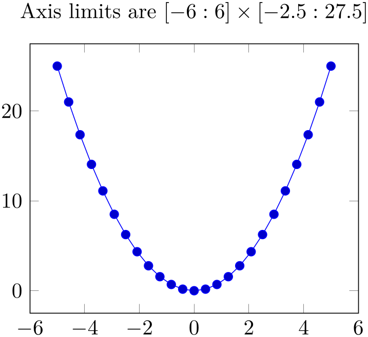
% Preamble: \pgfplotsset{width=7cm,compat=1.18}
\begin{tikzpicture}
\begin{axis}[
% Show (automatically) computed limits:
title={
Axis limits are
$
[\pgfmathprintnumber{\pgfkeysvalueof{/pgfplots/xmin}}
:\pgfmathprintnumber{\pgfkeysvalueof{/pgfplots/xmax}}
] \times
[\pgfmathprintnumber{\pgfkeysvalueof{/pgfplots/ymin}}
:\pgfmathprintnumber{\pgfkeysvalueof{/pgfplots/ymax}}
]$ },
]
\addplot {x^2};
\end{axis}
\end{tikzpicture}
This access is possible inside of any axis description (like
xlabel, title, legend entries, etc.) or any annotation (i.e. inside of \node, \draw or
\path and coordinates in (x,y)), but not inside of \addplot (limits may not
be complete at this stage).
-
/pgfplots/xmode=normal|linear|log (initially normal)
-
/pgfplots/ymode=normal|linear|log (initially normal)
-
/pgfplots/zmode=normal|linear|log (initially normal)
Allows to choose between linear (= normal) or logarithmic axis scaling or log plots for each \(x,y,z\)-combination.
Logarithmic plots use the current setting of log basis x and its variants to determine the basis (default is \(e\)).
-
/pgfplots/x dir=normal|reverse (initially normal) 
-
/pgfplots/y dir=normal|reverse (initially normal) 
-
/pgfplots/z dir=normal|reverse (initially normal) 
Allows to reverse axis directions such that values are given in decreasing order.
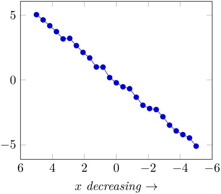
% Preamble: \pgfplotsset{width=7cm,compat=1.18}
\begin{tikzpicture}
\begin{axis}[
                        xlabel=$x$
                    \emph{decreasing} $\to$,
x dir=reverse,
]
                        \addplot {x
                    + rand*0.3};
\end{axis}
\end{tikzpicture}
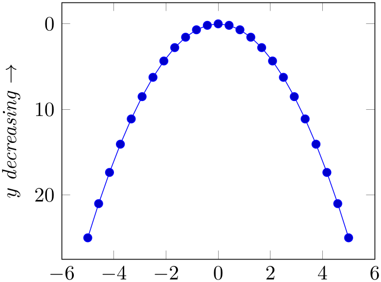
% Preamble: \pgfplotsset{width=7cm,compat=1.18}
\begin{tikzpicture}
\begin{axis}[
                        ylabel=$y$
                    \emph{decreasing} $\to$,
y dir=reverse,
]
\addplot {x^2};
\end{axis}
\end{tikzpicture}
Note that axis descriptions and relative positioning macros will stay at the same place as they would for non-reversed axes.
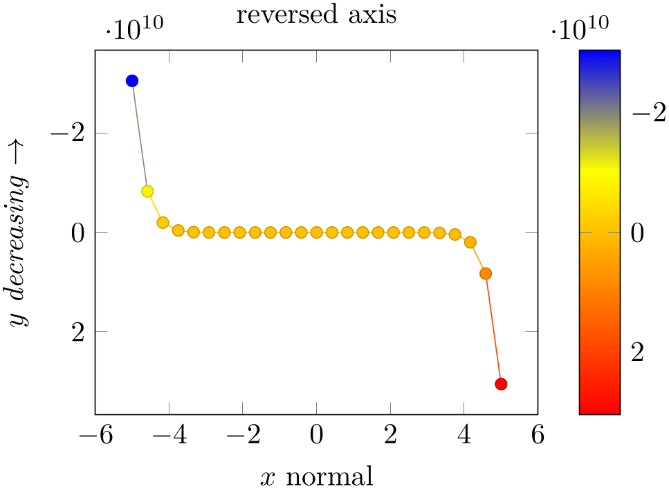
% Preamble: \pgfplotsset{width=7cm,compat=1.18}
\begin{tikzpicture}
\begin{axis}[
ylabel=$y$ \emph{decreasing} $\to$,
xlabel=$x$ normal,
title=reversed axis,
y dir=reverse,
colorbar,
colorbar style={y dir=reverse},
]
                            \addplot+
                    [mesh,scatter] {x^15};
\end{axis}
\end{tikzpicture}
Note that colorbars won’t be reversed automatically, you will have to reverse the sequence of color bars manually in case this is required as in the preceding example.
-
/pgfplots/clip xlimits=true|false (initially true) 
-
/pgfplots/clip ylimits=true|false (initially true) 
-
/pgfplots/clip zlimits=true|false (initially true) 
-
/pgfplots/clip limits=true|false 
Configures what to do if some, but not all axis limits have been specified explicitly. In case clip limits=true, the automatic limit computation will only consider points which do not contradict the explicitly set limits.
The effect of clip xlimits=true is that if the \(x\)-coordinate of some point \((x,y)\) falls outside of the limits specified by xmin and xmax, neither \(x\) nor \(y\) will contribute to the automatically computed axis limits. The key clip limits is an alias which sets all the other options at once.
This option has nothing to do with path clipping, it only affects how the axis limits are computed.
-
/pgfplots/enlarge x limits=auto|true|false|upper|lower|
 val
val |value=val|abs value=val|
abs=val|rel=val (initially auto)
-
/pgfplots/enlarge y limits=auto|true|false|upper|lower|
val|value=val|abs value=val|
abs=val|rel=val (initially auto)
-
/pgfplots/enlarge z limits=auto|true|false|upper|lower|
val|value=val|abs value=val|
abs=val|rel=val (initially auto)
-
/pgfplots/enlargelimits=
common value
Enlarges the axis size for one axis (or all of them for enlargelimits) somewhat if enabled.
You can set xmin, xmax and ymin, ymax to the minimum/maximum values of your data and enlarge x limits will enlarge the canvas such that the axis doesn’t touch the plots.
The value true enlarges the lower and upper limit.
The value false uses tight axis limits as specified by the user (or read from input coordinates).
The value auto will enlarge limits only for axis for which axis limits have been determined automatically. For three-dimensional figures, the auto mechanism applies only for the \(z\)-axis. The \(x\)- and \(y\)-axis won’t be enlarged.
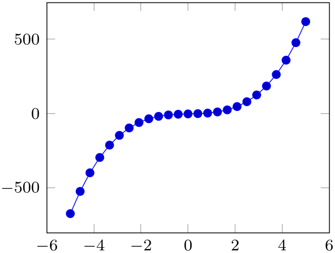
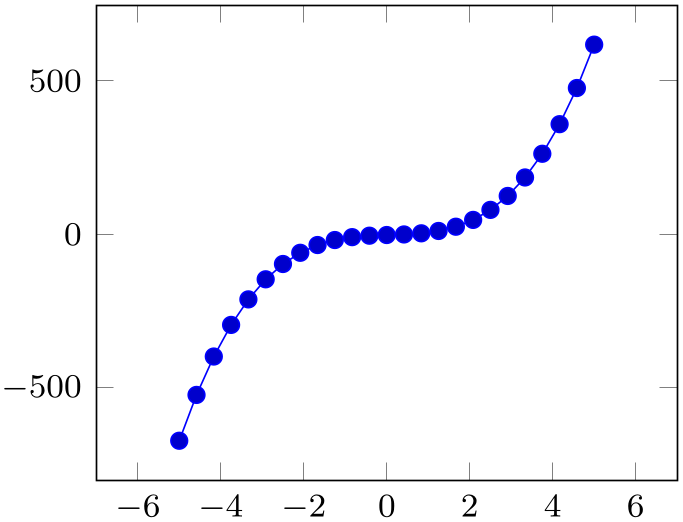
% Preamble: \pgfplotsset{width=7cm,compat=1.18}
\begin{tikzpicture}
\begin{axis}[
small,
]
                        \addplot {5 * x^3 - x^2 + 4*x
                    -2};
\end{axis}
\end{tikzpicture}
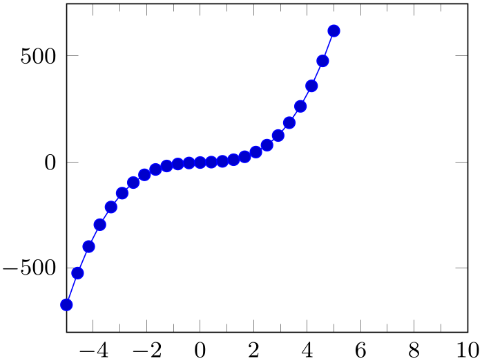
Specifying a number value like ‘enlarge x limits=0.2’ will enlarge lower and upper axis limit relatively. The following example adds \(20\%\) of the axis limits on both sides:
% Preamble: \pgfplotsset{width=7cm,compat=1.18}
\begin{tikzpicture}
\begin{axis}[
small,
enlarge x limits=0.2,
]
                        \addplot {5 * x^3 - x^2 + 4*x
                    -2};
\end{axis}
\end{tikzpicture}
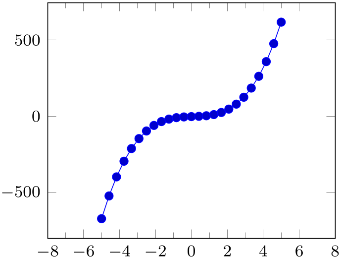
The choice rel={value} is the same as true,value={value}, i.e. it activates relative enlargement for both upper and lower limit.
The value upper enlarges only the upper axis limit while
lower enlarges only the lower axis limit. In this case, the
amount added to the respective limit can be specified using the
value={val} key. It can be combined with any of the other possible values. For example,
\pgfplotsset{enlarge x limits={value=0.2,upper}}
will enlarge (only) the upper axis limit by \(20\%\) of the axis range. Another example is
\pgfplotsset{enlarge x limits={value=0.2,auto}}
which changes the default threshold of the auto value to \(20\%\).
% Preamble: \pgfplotsset{width=7cm,compat=1.18}
\begin{tikzpicture}
\begin{axis}[
small,
minor x tick num=1,
enlarge x limits={rel=0.5,upper},
]
                        \addplot {5 * x^3 - x^2 + 4*x
                    -2};
\end{axis}
\end{tikzpicture}
While value uses relative thresholds,
abs value accepts absolute values: it adds an absolute
value to the selected axis. The choice abs={value} is the same as true,abs value={value}, i.e. it adds an absolute value to both upper and lower limit:
% Preamble: \pgfplotsset{width=7cm,compat=1.18}
\begin{tikzpicture}
\begin{axis}[
small,
minor x tick num=1,
enlarge x limits={abs=3},
]
                        \addplot {5 * x^3 - x^2 + 4*x
                    -2};
\end{axis}
\end{tikzpicture}
Here, we enlarged by \(3\) units of the \(x\)-axis. Note that you can also specify dimensions like 1cm:
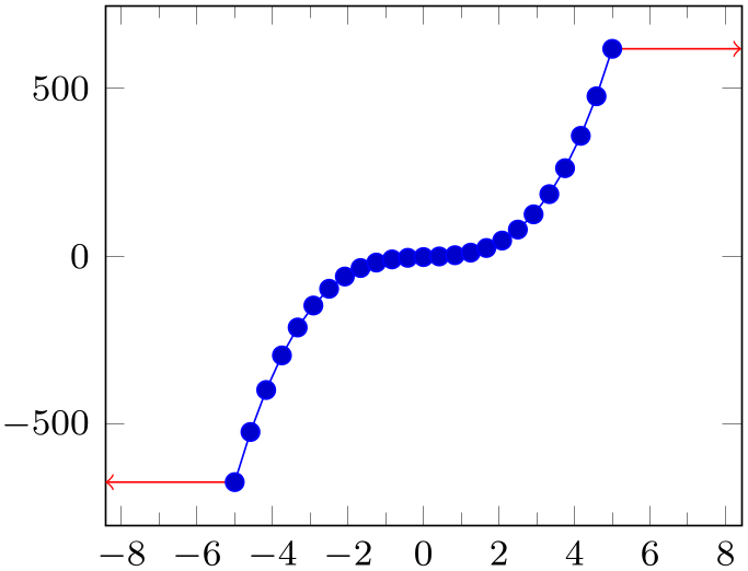
% Preamble: \pgfplotsset{width=7cm,compat=1.18}
\begin{tikzpicture}
\begin{axis}[small,minor x tick num=1,
enlarge x limits={abs=1cm},
]
                        \addplot {5 * x^3 - x^2 + 4*x
                    -2}
coordinate [pos=0] (first)
coordinate [pos=1] (last);
\draw [red,->] (first) -- ++(-1cm,0pt);
\draw [red,->] (last) -- ++( 1cm,0pt);
\end{axis}
\end{tikzpicture}
Technically, the use of absolute dimensions is a little bit different. For example, it allows to enlarge by more than width which is impossible for all other choices. pgfplots will try to fulfill both the provided width/height and the absolute axis enlargements. If it fails to do so, it will give up on width/height constraints and print a warning message to your logfile. See also the key enlargelimits respects figure size.
abs value is applied multiplicatively for logarithmic axes! That means abs value=10 for a logarithmic axis adds \(\log 10\) to upper and/or lower axis limits.
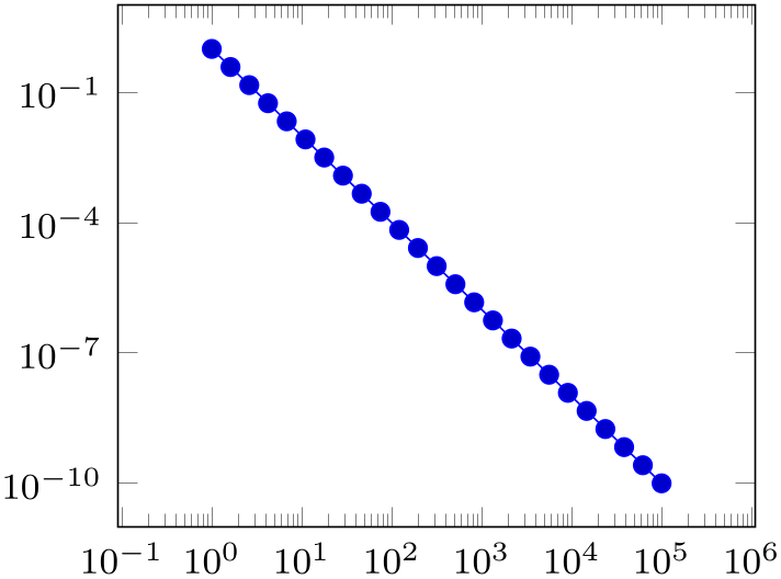
% Preamble: \pgfplotsset{width=7cm,compat=1.18}
\begin{tikzpicture}
\begin{loglogaxis}[
small,
enlarge x limits={abs=11},
]
\addplot+ [domain=1:100000] {x^-2};
\end{loglogaxis}
\end{tikzpicture}
Note that enlargelimits is applied before any changes to axis limits are considered as part of scale mode: enlargelimits will always be applied. Afterwards, the choice scale mode=scale uniformly will enlarge limits once more in order to satisfy all scaling constraints. The two limit enlargements are independent of each other, i.e. even if you say enlargelimits=false, scale mode will still increase axis limits if this seems to be necessary. An exception for this rule is enlarge-by-dimension, i.e. something like abs=1cm (see enlargelimits respects figure size for this case). See scale mode (especially scale mode=units only) and unit rescale keep size for detail on how to disable limit enlargement caused by scale mode.
-
/pgfplots/enlargelimits respects figure size=true|false (initially true) 
A key which is only used for something like enlarge x limits={abs=1cm}, i.e. for enlarge-by-dimension. It controls if pgfplots will try to respect width/height. You should probably always leave it as its default unless you run into problems.
If pgfplots fails to respect the figure size, it will print a warning message of sorts “enlargelimits respects figure size=true: could not respect the prescribed width/height” to your logfile.
-
/pgfplots/log origin x=0|infty (initially infty) 
-
/pgfplots/log origin y=0|infty (initially infty) 
-
/pgfplots/log origin z=0|infty (initially infty) 
-
/pgfplots/log origin=0|infty (initially infty) 
Allows to choose which coordinate is the logical “origin” of a logarithmic plot (either for a particular axis or for all of them).
The choice log origin=infty is probably useful for stacked plots: it defines the “origin” in log coordinates to be \(-\infty \). To be compatibly with older versions, this is the default. Note that \(-\infty \) is clipped to be the lowest displayed value on the axis in question.
The choice log origin=0 defines the logarithmic origin to be the natural choice \(\log (1)=0\). This is particularly useful for ycomb plots.
-
\begin{pgfplotsinterruptdatabb} 
-
environment contents
-
\end{pgfplotsinterruptdatabb} 
Everything in
environment contents
will not contribute to the data bounding box.
The same effect can be achieved with update limits=false inside curly braces.
4.14.2Accessing Computed Limit Ranges
This section is for those who want or need to access the computed limits programmatically. It lists how to access computed values.
-
/pgfplots/xmin(no value)
-
/pgfplots/ymin(no value)
-
/pgfplots/zmin(no value)
-
/pgfplots/xmax(no value)
-
/pgfplots/ymax(no value)
-
/pgfplots/zmax(no value)
These values are not only the input: after the survey phase, their values will be overwritten with the resulting computed values. These may differ according to enlargelimits or scale mode.
If you need to access them, you can write \pgfkeysvalueof{/pgfplots/xmin} somewhere in your code.