Manual for Package pgfplots
2D/3D Plots in LATeX, Version 1.18.2
https://github.com/pgf-tikz/pgfplots
The Reference
4.8Providing Color Data – Point Meta
pgfplots provides features which modify plots depending on a special coordinate, the “point meta data”. For example, scatter plots may vary marker colors, size or appearance depending on this special data. Surface and mesh plots are another example: here, the color of a surface patch (or mesh part) depends on “point meta”. The “meta data” of a node is not the position (which is given as \((x,y)\) or \((x,y,z)\)). It is “some information” about that node; you could say: it is a specific property of the node. This is commonly called “meta data”.
4.8.1Point Meta Overview
In pgfplots, every node has its coordinate and its meta data. Thus, two-dimensional plots have three values: \(x\), \(y\), and the point meta data. Three-dimensional plots have four values for each coordinate: \(x\), \(y\), \(z\), and the point meta.
In many cases, point meta is interpreted to be color data. To be more precise: it is interpreted to be scalar color data which is mapped into the colormap (more about this approach in the next paragraphs). However, point meta can be anything. Often, it is a single number as in the case of color data. That number is mapped linearly to the interval \([0,1000]\) such that \(0\) corresponds to the smallest encountered value and \(1000\) corresponds to the largest encountered scalar value. The mapped value is available as \pgfplotspointmetatransformed. This special value allows to define some property of the plot: it can be the color (together with colormap). It can also be the line width in a mesh plot (more precisely: the line width could be defined to depend on the transformed meta data). An example for this approach is on page (page for section 4.5.8) where a quiver plot’s arrow line with depends on \pgfplotspointmetatransformed. The value can also be used to define mark size as in the example for scatter/@pre marker code on page (??). However, point meta data does not necessarily need to be a number. It can be a text label (any text that you like). This is used by nodes near coords, for example. It could also contain a tuple like RGB color information (compare mesh/color input=explicit). Thus, point meta is really some abstract information about individual coordinates.
Note that there is only one point meta per point. See the key visualization depends on if you need more than one meta data value per coordinate.
The common idea is to tell pgfplots how to get the meta data. It is not necessary to provide data explicitly – in many cases, the data which is used to color surface patches or marker colors is the plot’s \(y\) or \(z\) coordinate. The method used to tell pgfplots where to find “point meta data” is the point meta key.
The most common use case of point meta is color information: if the point meta data is in the interval \([m_{\min },m_{\max }]\), the point meta coordinate for the smallest encountered value \(m = m_{\min }\) will get the lowest color provided by the colormap while the largest encountered value \(m=m_{\max }\) will get the highest color provided by the colormap. As already mentioned, this is accomplished using \pgfplotspointmetatransformed \(\in [0,1000]\) (per convention). Any coordinate between the smallest and largest values will be mapped linearly: for example, the mean \(m = 1/2 (m_{\max } + m_{\min })\) will get the middle color of the color map (it will have \pgfplotspointmetatransformed \(=500\)). This is why “point meta” is sometimes called “color data” in this manual.
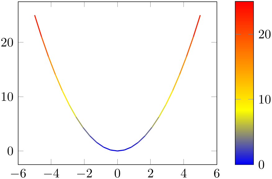
% Preamble: \pgfplotsset{width=7cm,compat=1.18}
\begin{tikzpicture}
\begin{axis}[colorbar]
\addplot [mesh,point meta=y,thick] {x^2};
\end{axis}
\end{tikzpicture}
4.8.2User Input Format for Point Meta
-
/pgfplots/point meta=none|
 expression
 |x|y|z|f(x)|explicit|explicit symbolic (initially none)
-
none The initial choice none disables point meta data, resulting in no computational work. Any other choice will activate the computation of upper and lower ranges for point meta data, i.e. the computation of \([m_{\min },m_{\max }]\).
-
x The choice x uses the already available \(x\) coordinates as point meta data. This does always refer to the final \(x\)-coordinates after any user transformations, logarithms, stacked plot computations, etc. have been applied. Consider using rawx if you need the unprocessed coordinate value here.
-
y
-
z The choices y and z are similar: they use the \(y\)- or \(z\)-coordinates respectively as point meta data. Consequently, these three choices do not need any extra data. As for x, there are math constants rawy and rawz which yield the unprocessed \(y\) and \(z\) value, respectively.
-
f(x) This will use the last available coordinate, in other words: it is the same as y for two dimensional plots and z for three dimensional ones.
-
explicit This choice tells pgfplots to expect numerical point meta data which is provided explicitly in the coordinate input streams. This data will be transformed linearly into the current color map as it has been motivated above.
How point meta data is provided for \addplot coordinates, \addplot table and the other input methods is described in all detail in Section 4.3.1 – but we provide small examples here to summarize the possibilities:
% for 'coordinates':% provide color data explicitly using []% behind coordinates:\addplot+ [point meta=explicit]coordinates {(0,0) [1.0e10](1,2) [1.1e10](2,3) [1.2e10](3,4) [1.3e10]% ...};% for 'table':% Assumes a datafile.dat like% xcolname ycolname colordata% 0 0 0.001% 1 2 0.3% 2 2.1 0.4% 3 3 0.5% ...% the file may have more columns.\addplot+ [point meta=explicit]table [x=xcolname,y=ycolname,meta=colordata]{datafile.dat};% or, equivalently (perhaps a little bit slower):\addplot+ [point meta=\thisrow{colordata}]table [x=xcolname,y=ycolname]{datafile.dat};% for 'file':% Assumes a datafile.dat like% 0 0 0.001% 1 2 0.3% 2 2.1 0.4% 3 3 0.5% ...% the first three columns will be used here as x,y and meta,% resp.\addplot+ [point meta=explicit]file {datafile.dat};% 'table' using expressions which may depend on all% columns:% Assumes a datafile.dat like% xcolname ycolname anything othercol% 0 0 4 15% 1 2 5 20% 2 2.1 8 30% 3 3 42 40% ...% the file may have more columns.\addplot+ [point meta={0.5*(\thisrow{anything} + sqrt(\thisrow{othercol}))}]table [x=xcolname,y=ycolname]{datafile.dat};Thus, there are several methods to provide point meta (color data). The key for the choice explicit is that some data is provided explicitly – although point meta does not know how. The data is expected to be of numerical type and is mapped linearly into the range \([0,1000]\) (maybe for use in the current color map).
-
explicit symbolic The choice explicit symbolic is very similar to explicit in that it expects extra data by the coordinate input routines. However, explicit symbolic does not necessarily expect numerical data: you can provide any sort of symbols. One might provide a set of styles, one for each class in a scatter plot. This is implemented using scatter/classes, see page (page for section 4.5.12). Input data is provided in the same fashion as mentioned above for the choice explicit.
This choice is usedful for nodes near coords with textual labels (see page (??)) and for surface plots with explicit color (see mesh/color input=explicit for details).
-
 expression
 This choice allows to compute point meta data using a mathematical expression. The
 expression
 may depend on x, y, z which yield the current \(x\)-, \(y\)- or
\(z\)-coordinate, respectively. The coordinates are completely processed (transformations, logs) as mentioned above for
the choice x. Furthermore, the
 expression
 may depend on commands which are valid during
\addplot like
\plotnum or
\coordindex (see Section 4.25
for details). If coordinates are provided using
\addplot table, the macro \thisrow{
 colname
 } is particularly useful as it allows to access the value of the provided
 colname
 of the “current” row. Computations are performed using the floating point unit of
pgf, and all supported arithmetical operations can be used.
In essence, the
 expression
 may depend on everything which is known to all
\addplot commands: the \(x\), \(y\) and (if any) \(z\)
coordinates. In addition, it may depend upon rawx, rawy or
rawz. These three expressions yield the unprocessed \(x\), \(y\) or \(z\) value as it has been found in the input stream
(no logs, no user transformations).42 If used together with
\addplot table, you may also access other table columns (for example with
\thisrow{
 colname
 }).
}).
-
TeX code=
 code
code A rather low level choice which allows to provide
TeX
 code
code to compute a numerical value. The
 code
code should define the macro \pgfplotspointmeta. It is evaluated in a locally scoped environment (it’s local variables are freed afterwards). It may depend on
the same values as described for
 expression
 above, especially on \thisrow{
 colname
 } for table input.
Note that the math parser will be configured to use the fpu at this time, so \pgfmathparse yields floats.
Note that you need an extra pair of braces to provide this key, i.e.
point meta={TeX code={
 code
code }}.
}}.
-
TeX code symbolic=
 code
code Just as TeX code, you can provide
 code
code which defines the macro \pgfplotspointmeta, but the result is not interpreted as a number. It is like the explicit symbolic choice.
Note that you need an extra pair of braces to provide this key, i.e.
point meta={TeX code symbolic={
 code
code }}.
}}.
-
symbolic=
 symbol
 A choice which accepts some arbitrary
 symbol
 which is used for every coordinate. As explicit symbolic and TeX code symbolic, this choice yields
symbolic representations, i.e. it is kept as is without mapping the result.
The difference to explicit symbolic is that
 symbol
 is a common symbol for all points whereas explicit symbolic expects the input data stream (like a table) to
provide individual symbols.
The different to TeX code symbolic is marginal: symbolic is actually the same as
point meta/TeX code symbolic={\def\pgfplotspointmeta{
 symbol
 }}.
}}.
A use case for symbolic is mesh/color input=explicit mathparse, see the documentation there-in.
Note that you need an extra pair of braces to provide this key, i.e.
point meta={symbolic={
 symbol
 }}.
}}.
The point meta key tells pgfplots where to get the special point meta data. Please note that point meta and scatter src is actually the same – scatter src is an alias for point meta. Thus, the summary provided for scatter src on page (page for section 4.5.12) covers the same topics. However, the main reference for point meta is here.
As already mentioned, a main application of point meta data is to determine (marker/face/edge) colors using a linear map into the range \([0,1000]\) (maybe for use in the current color map). This map works as follows: it is a function
\[ \phi \colon [m_{\min },m_{\max }] \to [0,1000] \]
with
\[ \phi (m) = \frac {m - m_{\min }}{m_{\max } - m_{\min }} \cdot 1000 \]
such that \(\phi (m_{\min }) = 0\) and \(\phi (m_{\max })=1000\). The value \(1000\) is – per convention – the upper limit of all color maps. Now, if a coordinate (or edge/face) has the point meta data \(m\), its color will be determined using \(\phi (m)\): it is the color at \(\phi (m)\)‰ of the current color map.
This transformation depends on the interval \([m_{\min },m_{\max }]\) which, in turn, can be modified using the keys point meta rel, point meta min and point meta max described below.
The untransformed point meta data is available in the macro \pgfplotspointmeta (only in the correct context, for example the scatter plot styles or the scatter/@pre marker code interface). This macro contains a low level floating point number (unless it is non-parsed string data). The transformed data will be available in the macro \pgfplotspointmetatransformed and is in fixed point representation. It is expected to be in the range \([0,1000]\).
-
/pgfplots/set point meta if empty={
 point meta source
 }
}
Sets
point meta= point meta source
 , but only if
point meta=none
currently. This is used for scatter, mesh and
surf with
set point meta if empty=f(x).
42 In rare circumstances, it might be interesting to apply a math expression to another source of point meta
(one of the other choices). To this end, the
 expression
 is checked after the other possible choices have already been evaluated. In other words, the statement
point meta=explicit, point meta=meta*meta+3 will evaluate the expression with meta set to whatever data
has been provided explicitly.
4.8.3Mapping Point Meta and Color Maps
As already explained in the documentation for point meta, one application for point meta data is to determine colors using the current color map and a linear map from point meta data into the current color map. This subsection shows keys to control this mapping.
The plot handlers surf, mesh, patch, scatter, contour prepared, and some related ones all make use of mapped colors. To this end, the value provided by point meta is processed as follows:
-
• First, all encountered values are collected (during \addplot) and the largest and smallest value, \(m_{\max }\) and \(m_{\min }\), are computed. The value is stored in \pgfplotspointmeta.
-
• Second, every encountered value \(m\) is mapped to \([0,1000]\) using a linear map: \(m_{\min } \to 0\); \(m_{\max }\to 1000\), and all values in-between are mapped linearly. This value is stored (and available) in the TeX macro \pgfplotspointmetatransformed (but not before \end{axis}).
-
• Finally, the mapped value \pgfplotspointmetatransformed is mapped into the current colormap. The resulting color is called mapped color.
The plot handlers, in turn, use mapped color in order to render their colors (often combined with color mixins like mapped color!80!black).
-
/pgfplots/point meta rel=axis wide|per plot (initially axis wide) 
The key point meta rel configures whether the interval of all point meta coordinates, \([m_{\min },m_{\max }]\) is computed as maximum over all plots in the complete axis (the choice axis wide) or only for one particular plot (the choice per plot).
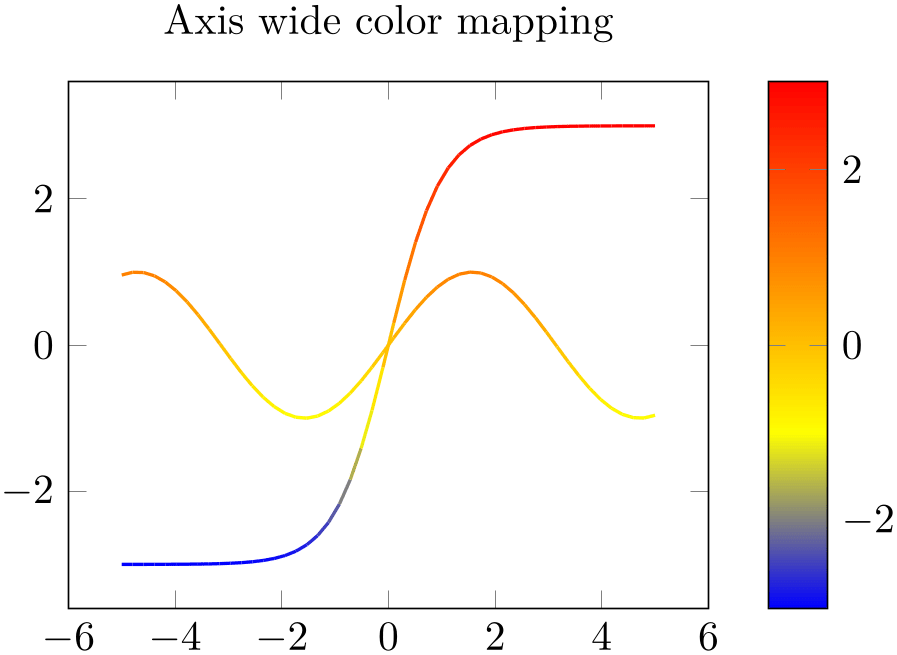
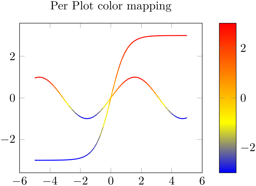
% Preamble: \pgfplotsset{width=7cm,compat=1.18}
\begin{tikzpicture}
\begin{axis}[
title=Axis wide color mapping,
colorbar,
                            samples=50,point meta rel=axis
                    wide,
point meta=y,
]
\addplot [mesh,thick] {sin(deg(x))};
\addplot [mesh,thick] {3*tanh(x)};
\end{axis}
\end{tikzpicture}
~
\begin{tikzpicture}
\begin{axis}[
title=Per Plot color mapping,
colorbar,
samples=50,
point meta rel=per plot,
point meta=y,
]
\addplot [mesh,thick] {sin(deg(x))};
\addplot [mesh,thick] {3*tanh(x)};
\end{axis}
\end{tikzpicture}
Note that a colorbar will still use the axis wide point meta limits. Consider the colorbar source key if you want the color data limits of a particular plot for your color bar. The point meta rel key configures how point meta maps to colors in the colormap.
-
/pgfplots/point meta min={
 number
 }
}
-
/pgfplots/point meta max={
 number
 }
}
These keys allow to define the range required for the linear map of point meta data into the range \([0,1000]\) (for example, for current maps) explicitly. This is necessary if the same mapping shall be used for more than one axis.
-
• It is possible to provide limits partially; in this case, only the missing limit will be computed.
-
• If point meta data falls outside of these limits, the linear transformation is still well defined which is acceptable (unless the interval is of zero length). However, color data can’t be outside of these limits, so color bars perform a truncation.
-
• This key can be provided for single plots as well as for the complete axis (or for both).
-
• If meta limits are provided for a single plot, these limits may also contribute to the axis wide meta interval.
-
/pgfplots/colormap access=map|direct|const|
piecewise constant|piecewise const|piecewise linear (initially map) 
This key configures how point meta data is used to determine colors from a color map.
4.8.3.1Mapping Point Meta using Piecewise Constant Interpolation
The initial configuration map performs the linear mapping operation explained above in all detail.
4.8.3.2Using Colormaps as Indexed Color Space (Palette)
The choice direct does not perform any transformation; it interprets the value of point meta as integer indices into the current color map. If a number is no integer, it will be truncated by throwing away any fraction parts of the number. Consequently, it is quite similar to index of colormap.
Suppose we have the color definitions
 RdPu-K,
 RdPu-I,
 RdPu-G,
 RdPu-E, and
 RdPu-B (which are actually taken from
\usetikzlibrary{colorbrewer}).
We will use these colors in order to define a colormap:
% Preamble: \pgfplotsset{width=7cm,compat=1.18}
% requires \usetikzlibrary{colorbrewer}
\begin{tikzpicture}
\begin{axis}[
colormap={brewer}{
color=(RdPu-B) color=(RdPu-E)
color=(RdPu-G) color=(RdPu-I)
color=(RdPu-K)
},
enlargelimits=false,
colorbar as palette,
]
\addplot [
matrix plot,
nodes near coords,mark=*,
point meta=explicit,
colormap access=direct,
] coordinates {
(0,0) [0] (1,0) [1] (2,0) [2] (3,0) [NaN]
(0,1) [3] (1,1) [4] (2,1) [5] (3,1) [99]
(0,2) [3.5] (1,2) [-1] (2,2) [2.99] (3,2) [3]
};
\end{axis}
\end{tikzpicture}
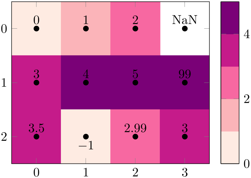
The example has a \(3\times 4\) matrix, each with explicitly provided values of
point meta. The first point has a point meta value of \(0\) and
uses the first color of the colormap (RdPu-B,
 ). The second point has value \(1\) and uses the second color, RdPu-E
 , and so on. Note that NaN is interpreted as ‘hole’ in the matrix and is left empty (you see the
background color here). Note furthermore that coordinate (1,2) [-1] is mapped to the first color since values
outside of the allowed range are automatically clipped to the next correct color. The same holds for the point with
[99]: it is mapped to the last available color
  . Finally, the point with [2.99] is mapped to index \(2\) (
 ) since colormap access=direct truncates to the next
integer index.
-
/pgfplots/colorbar as palette(no value) 
The example above makes use of colorbar as palette, a dedicated style useful for such palette-type applications.
It is defined as
\pgfplotsset{
colorbar as palette/.style={
colorbar sampled={
surf,
colormap access=direct,
shader=flat corner,
samples=\pgfplotscolormapsizeof
{\pgfkeysvalueof{/pgfplots/colormap name}}+1,
},
colorbar style={
point meta min=0,
point meta max=\pgfplotscolormapsizeof
{\pgfkeysvalueof{/pgfplots/colormap name}},
},
},
}
The idea is to show only the colors of the “palette”, i.e. without interpolating values of the colormap. Furthermore, it is supposed to show all available colors.
See also the closely related (but more general) colorbar as legend.
Note that colormap access=direct changes the way how point meta is translated to colors. However, it does not affect shader. In other words, it is perfectly sane to use shader=interp or shader=flat mean. This, however, will interpolate the colors resulting from colormap access=direct! Our example above uses shader=flat corner which results in no color interpolation at all.
The choice colormap access=direct is actually like a color palette for images with indexed colorspaces: suppose we use a random image of our choice, downsample it such that it does not become too large for LaTeX, and export it to coordinates of the form
1 1 194
1 2 194
1 3 170
1 4 193
1 5 188
1 6 188
...
with an indexed colorspace. Furthermore, we import its color palette as pgfplots colormap. To this end, a small Matlab script serves as utility to convert a tiff image to coordinates:43
[Z,cm] = imread('legoplane.tiff');
size(Z)
[X,Y]=meshgrid(1:size(Z,2), 1:size(Z,1));
data = [ X(:) Y(:) Z(:) ];
fid = fopen('legoplane.dat', 'w');
fprintf(fid, "% d %d %d\n", data');
fclose(fid);
fid = fopen('legoplane_cm.tex', 'w');
fprintf(fid, "\\pgfplotsset{colormap={legoplane palette}{\n");
fprintf(fid, "rgb=(% f,%f,%f)\n", cm');
fprintf(fid, "}}\n");
fclose(fid);
This allows us to import the graphics into pgfplots as matrix plot:

% Preamble: \pgfplotsset{width=7cm,compat=1.18}
\begin{tikzpicture}
% load and activate the CM:
\input{legoplane_cm.tex}
\begin{axis}[view={0}{90},axis equal,enlargelimits=false]
\addplot3 [
matrix plot,
colormap access=direct,
mesh/rows=128,
mesh/ordering=colwise,
] table {legoplane.dat};
\end{axis}
\end{tikzpicture}
The files legoplane_cm.tex, legopolane.dat, and legoplane.tiff are shipped with pgfplots and can be downloaded from CTAN. The keys to decode the table data into a mesh are specific to the Matlab export format of our script.
Note that rendering images from coordinates is considerably less efficient than \includegraphics in terms of
-
• computational time required by pgfplots,
-
• space consumption in the resulting pdf document,
-
• and time to render the resulting pdf in the viewer(s).
Depending on the use case, \addplot graphics may help to reduce typesetting times.
-
• If there are \(m\) colors in the color map and the color data falls outside of \([0,m-1]\), it will be pruned to either the first or the last color.
-
• If color data is a real number, it will be truncated to the next smaller integer.
-
• If colormap access=direct is combined with a shader\(\neq \)flat corner, color interpolation takes place. However, the color interpolation is not carried out in terms of the scalar point meta (as would have been done for colormap access=map). Instead, it is carried out on the resulting colors in their own colorspace.
-
• Note that patch refines or patch to triangles is unsupported in this context (at the time of this writing, it will interpolate the color indices, resulting in badly defined behavior).
See also the related keys color of colormap and index of colormap.
The choice colormap access=piecewise linear is an alias for colormap access=map. It is related to color of colormap.
43 Also see Section 8.2.1, “Importing Mesh Data From Matlab To PGFPlots” on page (page for section 8.2.1)
4.8.3.3Mapping Point Meta using Piecewise Constant Interpolation
The following paragraph makes uses of pdf features which are unsupported by some free viewers (including pdf.js and evince). Please resort to a suitable viewer if you see unexpected results.
The choice colormap access=piecewise constant is very similar to colormap access=map: it accepts the same point meta values as input, maps them linearly into \([0,1000]\) and uses the first color of the colormap if the value of point meta is point meta min and the last color of the colormap if the value of point meta is point meta max. However, values of point meta which fall between two colormap entries are interpolated using piecewise constant interpolation, i.e. just like const plot: the interpolated color resembles the value of the first color of the interval. As a consequence, the result contains at most as many colors as the colormap provides:
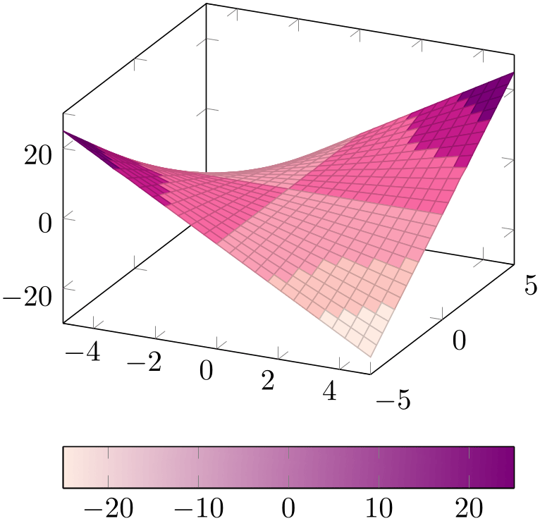
% Preamble: \pgfplotsset{width=7cm,compat=1.18}
% requires \usepgfplotslibrary{colorbrewer}
\begin{tikzpicture}
\begin{axis}[
                      colormap access=piecewise
                  constant,
colormap/RdPu-6,
colorbar horizontal,
]
\addplot3 [
surf,
] {x*y};
\end{axis}
\end{tikzpicture}
The choice colormap access=piecewise constant is compatible with all available shaders, but its best results are possible using shader=interp as this will avoid rectangular artifacts at mesh boundaries.
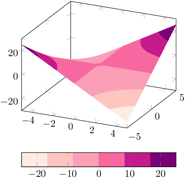
% Preamble: \pgfplotsset{width=7cm,compat=1.18}
% requires \usepgfplotslibrary{colorbrewer}
\begin{tikzpicture}
\begin{axis}[
                      colormap access=piecewise
                  constant,
colormap/RdPu-6,
colorbar horizontal,
]
\addplot3 [
surf,
shader=interp,
] {x*y};
\end{axis}
\end{tikzpicture}
The choice colormap access=piecewise constant requires colormaps with a suitable number of colors. This is quite different to colormap access=map (or piecewise linear) where the actual number of colors in the colormap cannot be seen in the resulting plot. In order to get the desired effects, one may need the same colormap with a different number of samples. To this end, one can make use of the special colormap syntax which is based on samples of colormap and its variants:
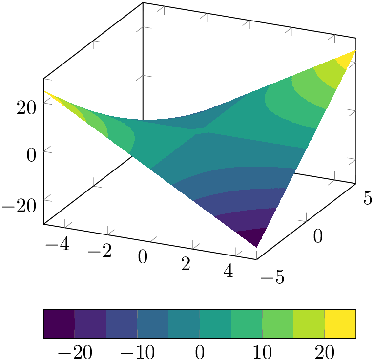
% Preamble: \pgfplotsset{width=7cm,compat=1.18}
\begin{tikzpicture}
\begin{axis}[
                      colormap access=piecewise
                  constant,
                      colormap={my sampled version of
                  viridis}{
samples of colormap=(10 of viridis)
},
colorbar horizontal,
]
\addplot3 [
surf,
shader=interp,
] {x*y};
\end{axis}
\end{tikzpicture}
The example takes the existing colormap name=viridis and chooses \(10\) samples of it. The result is called my sampled version of viridis and is used as “current colormap”. Details about this process can be read in Section 4.7.6.4 on page (page for section 4.7.6.4).
the plot handler contour filled which is based on such a visualization scheme.
The strategy which determines colors in this context is also available as const color of colormap.
The choices piecewise const and const are aliases for piecewise constant.