Manual for Package pgfplots
2D/3D Plots in LATeX, Version 1.18.2
https://github.com/pgf-tikz/pgfplots
The Reference
4.15Tick Options
4.15.1Tick Coordinates and Label Texts
-
/pgfplots/xtick distance={
 empty or numeric
 } (initially empty)
-
/pgfplots/ytick distance={
 empty or numeric
 } (initially empty)
-
/pgfplots/ztick distance={
 empty or numeric
 } (initially empty)
Allows to define the distance between generated tick positions.
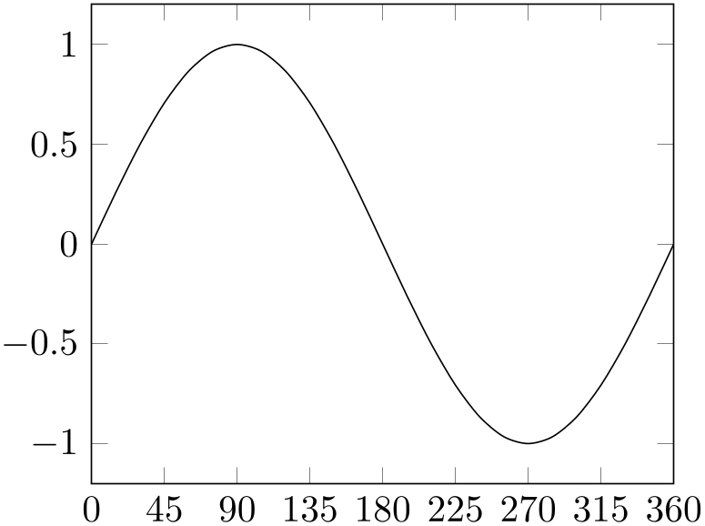
% Preamble: \pgfplotsset{width=7cm,compat=1.18}
\begin{tikzpicture}
\begin{axis}[
xtick distance=45,
ytick distance=0.5,
enlarge x limits=false,
]
\addplot [smooth,domain=0:360] {sin(x)};
\end{axis}
\end{tikzpicture}
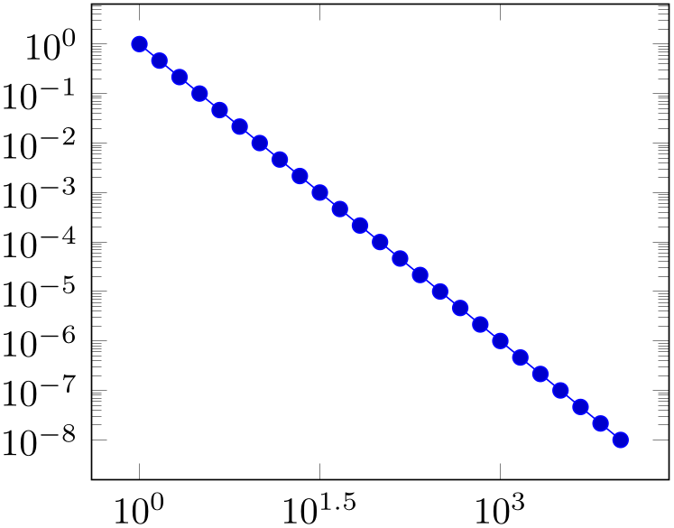
% Preamble: \pgfplotsset{width=7cm,compat=1.18}
\begin{tikzpicture}
\begin{loglogaxis}[
xtick distance=10^(1.5),
ytick distance=10^1,
]
                        \addplot expression
                    [domain=1:10000] {x^-2};
\end{loglogaxis}
\end{tikzpicture}
The initial value is empty meaning “generate as needed”.
Any other value is interpreted as constant (evaluated using the math expression parser) and is taken as is. Note that such values should be chosen in a way such that not too many and not too few tick positions are generated.
-
/pgfplots/xtick=\empty|data|{
 coordinate list
 } (initially
{
 })
})
-
/pgfplots/ytick=\empty|data|{
 coordinate list
 } (initially
{
 })
})
-
/pgfplots/ztick=\empty|data|{
 coordinate list
 } (initially
{
 })
})
-
• {0,1,2,5,8,1e1,1.5e1} (a series of coordinates),
-
• {0,...,5} (the same as {0,1,2,3,4,5}),
-
• {0,2,...,10} (the same as {0,2,4,6,8,10}),
-
• {9,...,3.5} (the same as {9, 8, 7, 6, 5, 4}),
-
• See [7, Section 34] for a more detailed definition of the options.
-
• Please be careful with white spaces inside of
 coordinate list
 (at least around the dots).
These
options assign a list of positions where ticks shall be placed. The argument is either the empty string (which is
the initial value), the command \empty, the special string ‘data’ or a list of
coordinates. The initial configuration of an empty string means to generate these positions automatically. The choice
\empty will result in no tick at all. The special value ‘data’ will produce tick marks at
every coordinate of the first plot. Otherwise, tick marks will be placed at every coordinate in
 coordinate list
 .
.
The
 coordinate list
 will be used inside of a \foreach \x in {
 coordinate list
 } statement. The format is as follows:
For log plots, pgfplots will apply \(\log (\cdot )\) to each element in ‘ coordinate list
 ’ (similarly, any custom transformations are applied to the argument list).
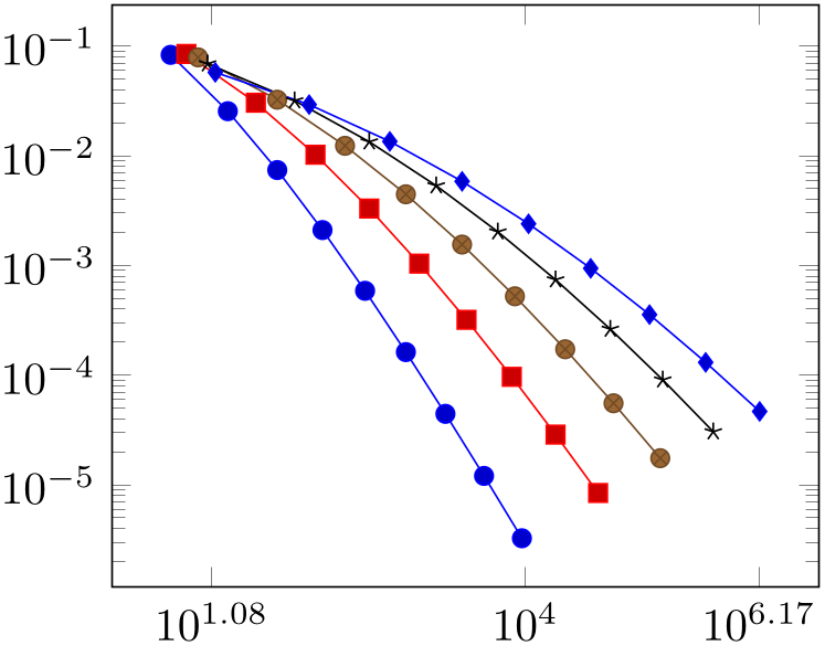
% Preamble: \pgfplotsset{width=7cm,compat=1.18}
\begin{tikzpicture}
\begin{loglogaxis}[
xtick={
12,
9897,
1468864
},
]
% see above for this macro:
\plotcoords
\end{loglogaxis}
\end{tikzpicture}
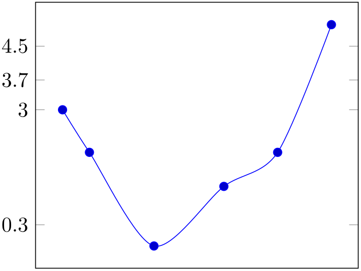
% Preamble: \pgfplotsset{width=7cm,compat=1.18}
\begin{tikzpicture}
\begin{axis}[
xtick=\empty,
ytick={-2,0.3,3,3.7,4.5},
]
\addplot+ [smooth] coordinates {
(-2,3) (-1.5,2) (-0.3,-0.2)
(1,1.2) (2,2) (3,5)
};
\end{axis}
\end{tikzpicture}
You can’t use the ‘...’ syntax if the elements are too large for TeX! For example, ‘xtick={1.5e5,2e7,3e8}’ will work (because the elements are interpreted as strings, not as numbers), but ‘xtick={1.5,3e5,...,1e10}’ will fail because it involves real number arithmetics beyond TeX’s capacities.
The default choice for tick positions in normal plots is to place a tick at each coordinate \(i\cdot h\). The step size \(h\) depends on the axis scaling and the axis limits. It is chosen from a list of “feasible” step sizes such that neither too much nor too few ticks will be generated. The default for log plots is to place ticks at positions \(10^i\) in the axis’ range. The positions depend on the axis scaling and the dimensions of the picture. If log plots contain just one (or two) positions \(10^i\) in their limits, ticks will be placed at positions \(10^{i\cdot h}\) with “feasible” step sizes \(h\) as in the case of linear axis.
The tick appearance can be (re)configured with
\pgfplotsset{tick style={very thin,gray}} % modifies the style `every tick'
                  \pgfplotsset{minor tick style={black}}      % modifies the style `every
                  minor tick'
These style commands can be used at any time. The tick line width can be configured with ‘major tick length’ and ‘minor tick length’.
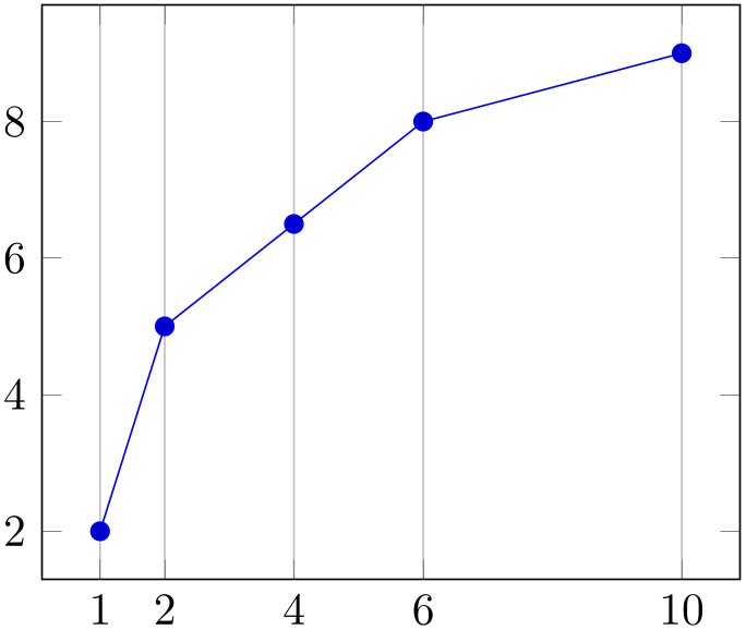
% Preamble: \pgfplotsset{width=7cm,compat=1.18}
\begin{tikzpicture}
\begin{axis}[
xtick=data,
xmajorgrids,
]
                      \addplot coordinates
                  {
(1,2)
(2,5)
(4,6.5)
(6,8)
(10,9)
};
\end{axis}
\end{tikzpicture}
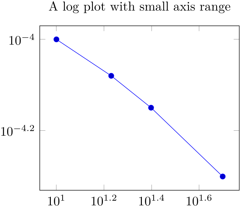
% Preamble: \pgfplotsset{width=7cm,compat=1.18}
\begin{tikzpicture}
\begin{loglogaxis}[
                      title=A log plot with small
                  axis range,
]
                      \addplot coordinates
                  {
(10,1e-4)
(17,8.3176e-05)
(25,7.0794e-05)
(50,5e-5)
};
\end{loglogaxis}
\end{tikzpicture}
-
/pgfplots/minor x tick num={
 number
 } (initially 0)
-
/pgfplots/minor y tick num={
 number
 } (initially 0)
-
/pgfplots/minor z tick num={
 number
 } (initially 0)
-
/pgfplots/minor tick num={
 number
 }
}
Sets the number of minor tick lines used either for single axes or for all of them.
Minor ticks will be disabled if the major ticks don’t have the same distance and they are currently only available for linear axes (not for logarithmic ones).

% Preamble: \pgfplotsset{width=7cm,compat=1.18}
\begin{tikzpicture}
\begin{axis}[
minor tick num=1,
]
\addplot {x^3};
\addplot {-20*x};
\end{axis}
\end{tikzpicture}
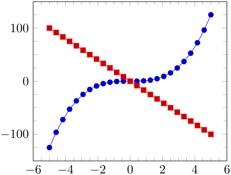
% Preamble: \pgfplotsset{width=7cm,compat=1.18}
\begin{tikzpicture}
\begin{axis}[
minor tick num=3,
]
\addplot {x^3};
\addplot {-20*x};
\end{axis}
\end{tikzpicture}

% Preamble: \pgfplotsset{width=7cm,compat=1.18}
\begin{tikzpicture}
\begin{axis}[
minor x tick num=1,
minor y tick num=3,
]
\addplot {x^3};
\addplot {-20*x};
\end{axis}
\end{tikzpicture}
-
/pgfplots/minor xtick=data|{
 coordinate list
 } (initially empty)
-
/pgfplots/minor ytick=data|{
 coordinate list
 } (initially empty)
-
/pgfplots/minor ztick=data|{
 coordinate list
 } (initially empty)
-
/pgfplots/minor tick=data|{
 coordinate list
 }
}
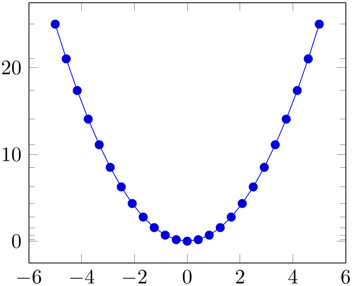
Allows to provide a list of minor tick positions manually. The syntax is almost the same as for xtick or ytick: simply provide either a comma-separated list of tick positions or the special value data. An empty argument argument disables the minor tick feature (in contrast to xtick where the special value \empty clears the list and an empty argument causes pgfplots to compute a default tick list).
In contrast to minor x tick num, this key allows to provide nonuniform minor tick positions.
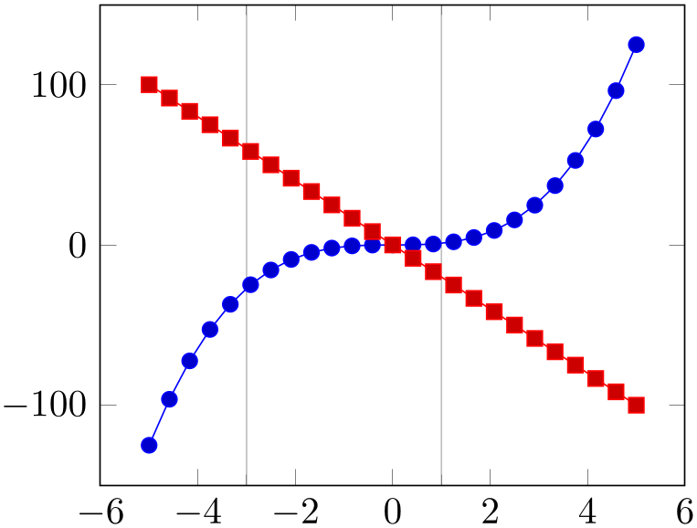
% Preamble: \pgfplotsset{width=7cm,compat=1.18}
\begin{tikzpicture}
\begin{axis}[
minor xtick={-3,1},
grid=minor,
]
\addplot {x^3};
\addplot {-20*x};
\end{axis}
\end{tikzpicture}
% Preamble: \pgfplotsset{width=7cm,compat=1.18}
\begin{tikzpicture}
\begin{axis}[
minor ytick=data,
]
\addplot {x^2};
\end{axis}
\end{tikzpicture}
This key has precedence over minor x tick num and its variants; if both of them are given, minor xtick is preferred and minor x tick num is ignored.
-
/pgfplots/extra x ticks={
 coordinate list
 }
}
-
/pgfplots/extra y ticks={
 coordinate list
 }
}
-
/pgfplots/extra z ticks={
 coordinate list
 }
}
-
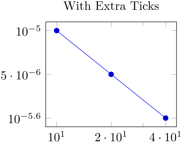
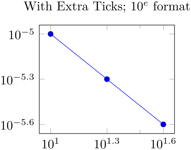
• Use extra x ticks to highlight special tick positions. The use of extra x ticks does not affect minor tick/grid line generation, so you can place extra ticks at positions \(j\cdot 10^i\) in log plots.
-
• Extra ticks are always typeset as major ticks.
They are affected by major tick length or options like grid=major.
-
• Use the style every extra x tick (every extra y tick) to configure the appearance.
-
• You can also use ‘extra x tick style={
 ...
... }’ which has the same effect.
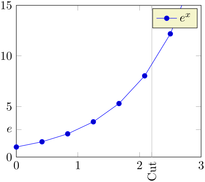
Adds additional tick positions and tick labels to the \(x\) or \(y\) axis. ‘Additional’ tick positions do not affect the normal tick placement algorithms, they are drawn after the normal ticks. This has two benefits: first, you can add single, important tick positions without disabling the default tick label generation and second, you can draw tick labels ‘on top’ of others, possibly using different style flags.
% Preamble: \pgfplotsset{width=7cm,compat=1.18}
\begin{tikzpicture}
\begin{axis}[
xmin=0,xmax=3,ymin=0,ymax=15,
extra y ticks={2.71828},
extra y tick labels={$e$},
extra x ticks={2.2},
extra x tick style={grid=major,
tick label style={
rotate=90,anchor=east}},
extra x tick labels={Cut},
]
\addplot {exp(x)};
\addlegendentry{$e^x$}
\end{axis}
\end{tikzpicture}

% Preamble: \pgfplotsset{width=7cm,compat=1.18}
\pgfplotsset{every axis/.append style={width=5.3cm}}
\begin{tikzpicture}
\begin{loglogaxis}[
title=Explicitly Provided Limits,
xtickten={1,2},
ytickten={-5,-6},
]
\addplot coordinates
{(10,1e-5) (20,5e-6) (40,2.5e-6)};
\end{loglogaxis}
\end{tikzpicture}
\begin{tikzpicture}
\begin{loglogaxis}[
title=With Extra Ticks,
xtickten={1,2},
ytickten={-5,-6},
extra x ticks={20,40},
extra y ticks={5e-6,2.5e-6},
]
\addplot coordinates
{(10,1e-5) (20,5e-6) (40,2.5e-6)};
\end{loglogaxis}
\end{tikzpicture}
\begin{tikzpicture}
\begin{loglogaxis}[
title=With Extra Ticks; $10^e$ format,
extra tick style={log identify minor tick positions=false},
xtickten={1,2},
ytickten={-5,-6},
extra x ticks={20,40},
extra y ticks={5e-6,2.5e-6},
]
\addplot coordinates
{(10,1e-5) (20,5e-6) (40,2.5e-6)};
\end{loglogaxis}
\end{tikzpicture}
Remarks:
-
/pgfplots/xtickten={
 exponent base 10 list
 }
}
-
/pgfplots/ytickten={
 exponent base 10 list
 }
}
-
/pgfplots/ztickten={
 exponent base 10 list
 }
}
These options allow to place ticks
at selected positions \(10^k\), \(k \in \) { exponent base 10 list
 }. They are only used for log plots. The syntax for {
 exponent base 10 list
 } is the same as above for xtick={
 list
list } or ytick={
 list
list }.
}.
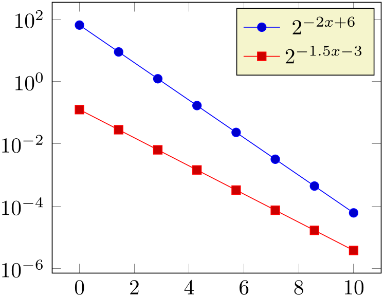
Using ‘xtickten={1,2,3,4}’ is equivalent to ‘xtick={1e1,1e2,1e3,1e4}’, but it requires fewer computational time and it allows to use the short syntax ‘xtickten={1,...,4}’.
% Preamble: \pgfplotsset{width=7cm,compat=1.18}
\begin{tikzpicture}
\begin{semilogyaxis}[
samples=8,
ytickten={-6,-4,...,4},
domain=0:10,
]
\addplot {2^(-2*x + 6)};
\addlegendentry{$2^{-2x + 6}$}
% or invoke gnuplot to generate coordinates:
                        \addplot gnuplot
                    [id=pow2]
{2**(-1.5*x -3)};
\addlegendentry{$2^{-1.5x -3}$}
\end{semilogyaxis}
\end{tikzpicture}
In case log basis x\(\,\neq 10\), the meaning of xtickten changes. In such a case, xtickten will still assign the exponent, but for the chosen log basis x instead of base \(10\).
-
/pgfplots/xticklabels={
 label list
 }
}
-
/pgfplots/yticklabels={
 label list
 }
}
-
/pgfplots/zticklabels={
 label list
 }
}
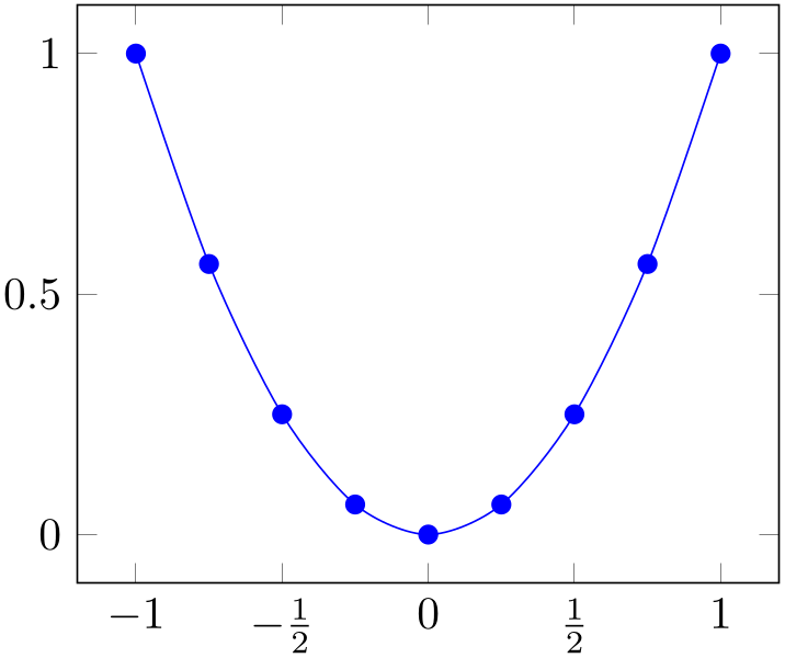
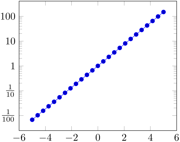
Assigns a list of tick labels to each tick position. Tick positions are assigned using the xtick and ytick options.
This is one of two options to assign tick labels directly. The other option is
xticklabel={ command
 } (or yticklabel={
 command
 }). The option ‘xticklabel’ offers higher flexibility while ‘xticklabels’ is easier to use. See also the variant
xticklabels from table.
The argument
 label list
 has the same format as for ticks, that means
xticklabels={$\frac{1}{2}$,$e$}
denotes the two element list \(\{\frac 12, e\}\). The list indices match the indices of the tick positions. If you need commas inside of list elements, use
xticklabels={{0,5}, $e$}.
% Preamble: \pgfplotsset{width=7cm,compat=1.18}
\begin{tikzpicture}
\begin{axis}[
xtick={-1.5,-1,...,1.5},
xticklabels={%
$-1\frac 12$,
$-1$,
$-\frac 12$,
$0$,
$\frac 12$,
$1$},
% note: \frac can be done automatically:
% xticklabel style={/pgf/number format/frac},
]
                        \addplot [smooth,blue,mark=*] coordinates
                    {
(-1, 1)
(-0.75, 0.5625)
(-0.5, 0.25)
(-0.25, 0.0625)
(0, 0)
(0.25, 0.0625)
(0.5, 0.25)
(0.75, 0.5625)
(1, 1)
};
\end{axis}
\end{tikzpicture}
% Preamble: \pgfplotsset{width=7cm,compat=1.18}
\begin{tikzpicture}
\begin{semilogyaxis}[
ytickten={-2,-1,0,1,2},
yticklabels={
$\frac{1}{100}$,
$\frac{1}{10}$,
1,10,100
},
]
\addplot {exp(x)};
\end{semilogyaxis}
\end{tikzpicture}
Note that it is also possible to terminate list entries with two backslashes, \\. In that case, the last entry needs to be terminated by \\ as well (it is the same alternative syntax which is also accepted for \legend and cycle list).
Please keep in mind that the arguments always refer the a list of tick positions, although it does not alter or
define the list of positions. Consequently, you should also provide the list of positions. Note that a list of positions
might be longer than what is actually displayed (in case the axis limits clip some of the value away), but the index mapping
into
 label list
 still includes the clipped values.
-
/pgfplots/xticklabel={
 command
 }
}
-
/pgfplots/yticklabel={
 command
 }
}
-
/pgfplots/zticklabel={
 command
 }
}
-
\ticknum The current tick number, starting with 0 (it is a macro containing a number).
-
\nexttick This command is only valid if the x tick label as interval option is set (or the corresponding variable for \(y\)). It will contain the position of the next tick position, that means the right boundary of the tick interval.
-
• \axisdefaultticklabel for normal plots:
-
• \axisdefaultticklabellog for log plots:
\def\axisdefaultticklabellog{%\pgfkeysgetvalue{/pgfplots/log number format code/.@cmd}\pgfplots@log@label@style\expandafter\pgfplots@log@label@style\tick\pgfeov}
These keys change the TeX command which creates the tick labels assigned to each tick position (see options xtick and ytick).
This is one of the two options to assign tick labels directly. The other option is ‘xticklabels={ label list
 }’ (or yticklabels={
 label list
 }). The option ‘xticklabel’ offers higher flexibility while ‘xticklabels’ is easier to use.
The argument
 command
 can be any
TeX
text. The following commands are valid inside of
 command
 :
:
The default argument is
That means you can configure the appearance of linear axis with the number formatting options described in Section 6.1.7 and logarithmic axis with log number format code, see below.
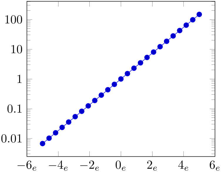
The key yticklabel is a code fragment which is supposed to handle any incoming \tick value. Consequently, it can be used to append custom suffixes or even units:
% Preamble: \pgfplotsset{width=7cm,compat=1.18}
\begin{tikzpicture}
\begin{semilogyaxis}[
log ticks with fixed point,
xticklabel={$\pgfmathprintnumber{\tick}_e$},
]
\addplot {exp(x)};
\end{semilogyaxis}
\end{tikzpicture}
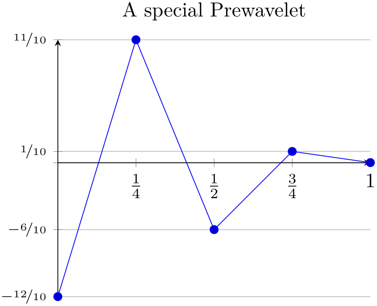
The following example uses explicitly formatted \(x\) tick labels and a small
TeX
script to format \(y\) tick labels as fractions in the form
 sign
sign
 number
 /10 (note that the
/pgf/number format/frac style can do similar
things automatically, see PgfplotsTable and the documentation therein).
% Preamble: \pgfplotsset{width=7cm,compat=1.18}
% \usepackage{nicefrace}% required
\begin{tikzpicture}
\begin{axis}[
% x ticks explicitly formatted:
xtick={0,1,0.5,0.25,0.75},
xticklabels={$0$,$1$,$\frac12$,$\frac14$,$\frac34$},
% y ticks automatically by some code fragment:
ytick=data,
yticklabel={
\scriptsize
\ifdim\tick pt<0pt % a TeX \if -- see TeX Book
\pgfmathparse{-10*\tick}
$-\nicefrac{\pgfmathprintnumber{\pgfmathresult}}{10}$
\else
\ifdim\tick pt=0pt
\else
\pgfmathparse{10*\tick}
$\nicefrac{\pgfmathprintnumber{\pgfmathresult}}{10}$
\fi
\fi
},
% NOTE: this here does the same:
% yticklabel style={/pgf/number format/.cd,frac,
% frac TeX=\nicefrac,frac whole=false,frac denom=10},
ymajorgrids,
title=A special Prewavelet,
axis x line=center,
axis y line=left,
]
\addplot coordinates {(0,-1.2) (0.25,1.1)
(0.5,-0.6) (0.75,0.1) (1,0)};
\end{axis}
\end{tikzpicture}
The TeX script takes the \tick macro as input and applies some logic. The \ifdim\tick pt<0pt means “if dimension \tick pt \(<\) 0pt”. The \ifdim is TeX’s only way to compare real fixed point numbers and the author did not want to invoke \pgfmath for this simple task. Since \ifdim expects a dimension, we have to use the pt suffix which is compatible with \pgfmath. The result is that negative numbers, zero and positive numbers are typeset differently.
You can change the appearance of tick labels with
\pgfplotsset{
% this modifies the `every tick label' style
tick label style={
font=\tiny,
/pgf/number format/sci,
},
}
and/or
\pgfplotsset{
% this modifies the `every x tick label' style
x tick label style={
above,
/pgf/number format/fixed zerofill,
},
}
and
-
/pgfplots/xticklabels from table={
 \table or filename
 }{
}{ colname
 }
}
-
/pgfplots/yticklabels from table={
 \table or filename
 }{
}{ colname
 }
}
-
/pgfplots/zticklabels from table={
 \table or filename
 }{
}{ colname
 }
}
A variant of
xticklabels={ list
list } which uses each entry in the column named
 colname
 from a table as tick labels.
The first argument
 \table or filename
 can be either a loaded table macro (i.e. the result of
\pgfplotstableread{
 file name
 }{
}{ \table
 }) or just a file name.
The second argument can be a column name, a column alias or a
create on use specification (see
PgfplotsTable for the latter two). Furthermore, it can be [index] integer
 in which case
 integer
 is a column index.
The behavior of
xticklabels from table is the same as
if the column
 colname
 would have been provided as comma separated list to
xticklabels. This means the column can contain text,
TeX
macros or even math mode.
If you have white spaces in your cells, enclose the complete cell in curly braces, {example cell}. The detailed input format for tables is discussed in \addplot table and in the documentation for PgfplotsTable.
-
/pgfplots/extra x tick label={
 TeX
code
 }
}
-
/pgfplots/extra y tick label={
 TeX
code
 }
}
-
/pgfplots/extra z tick label={
 TeX
code
 }
}
As xticklabel provides code to generate tick labels for each xtick, the key extra x tick label provides code to generate tick labels for every element in extra x ticks.
-
/pgfplots/extra x tick labels={
 label list
 }
}
-
/pgfplots/extra y tick labels={
 label list
 }
}
-
/pgfplots/extra z tick labels={
 label list
 }
}
As xticklabels provides explicit tick labels for each xtick, the key extra x tick labels provides explicit tick labels for every element in extra x ticks.
-
/pgfplots/x tick label as interval=true|false (initially false) 
-
/pgfplots/y tick label as interval=true|false (initially false) 
-
/pgfplots/z tick label as interval=true|false (initially false) 
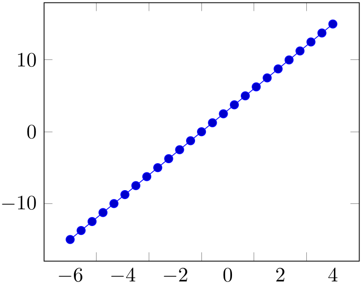
Allows to treat tick labels as intervals; that means the tick positions denote the interval boundaries. If there are \(n\) positions, \((n-1)\) tick labels will be generated, one for each interval.
% Preamble: \pgfplotsset{width=7cm,compat=1.18}
\begin{tikzpicture}
\begin{axis}[
x tick label as interval,
]
\addplot {3*x};
\end{axis}
\end{tikzpicture}
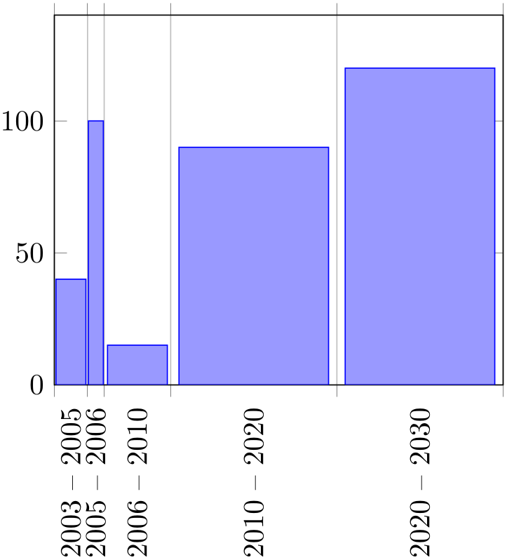
This mode enables the use of \nexttick inside of xticklabel (or yticklabel). A common application might be a bar plot.
% Preamble: \pgfplotsset{width=7cm,compat=1.18}
\begin{tikzpicture}
\begin{axis}[
ybar interval=0.9,
x tick label as interval,
xmin=2003,xmax=2030,
ymin=0,ymax=140,
xticklabel={
$\pgfmathprintnumber{\tick}$
-- $\pgfmathprintnumber{\nexttick}$},
xtick=data,
x tick label style={
rotate=90,anchor=east,
/pgf/number format/1000 sep=%
},
]
\addplot [draw=blue,fill=blue!40!white]
coordinates
{(2003,40) (2005,100) (2006,15)
(2010,90) (2020,120) (2030,3)};
\end{axis}
\end{tikzpicture}
-
/pgfplots/xminorticks=true|false (initially true) 
-
/pgfplots/yminorticks=true|false (initially true) 
-
/pgfplots/zminorticks=true|false (initially true) 
-
/pgfplots/xmajorticks=true|false (initially true) 
-
/pgfplots/ymajorticks=true|false (initially true) 
-
/pgfplots/zmajorticks=true|false (initially true) 
-
/pgfplots/ticks=minor|major|both|none (initially both) 
Enables/disables the small tick lines either for single axis or for all of them. Major ticks are those placed at the tick positions and minor ticks are between tick positions. Please note that minor ticks are automatically disabled if xtick is not a uniform range.60
The key minor tick length={ dimen
dimen } configures the tick length for minor ticks while the major variant applies to major ticks. You can configure
the appearance using the following styles:
\pgfplotsset{every tick/.append style={color=black}} % applies to major and minor ticks,
\pgfplotsset{every minor tick/.append style={thin}} % applies only to minor ticks,
\pgfplotsset{every major tick/.append style={thick}} % applies only to major ticks.
There is also the style “every tick” which applies to both, major and minor ticks.
-
/pgfplots/xtickmin={
 coord
coord }
}
-
/pgfplots/ytickmin={
 coord
coord }
}
-
/pgfplots/ztickmin={
 coord
coord }
}
-
/pgfplots/xtickmax={
 coord
coord }
}
-
/pgfplots/ytickmax={
 coord
coord }
}
-
/pgfplots/ztickmax={
 coord
coord }
}
These keys can be used to modify minimum/maximum values before ticks are drawn. Because this applies to axis discontinuities, it is described on page (??) in Section 4.9.12, “Axis Discontinuities”.
60 A uniform list means the difference between all elements is the same for linear axis or, for logarithmic axes, \(\log (10)\).
4.15.2Tick Alignment: Positions and Shifts
-
/pgfplots/xtick pos=lower|upper|bottom|top|left|right|both (initially both) 
-
/pgfplots/ytick pos=lower|upper|bottom|top|left|right|both (initially both) 
-
/pgfplots/ztick pos=lower|upper|bottom|top|left|right|both (initially both) 
-
/pgfplots/tick pos=lower|upper|bottom|top|left|right|both 
Allows to choose where to place the small tick lines. In the default configuration, this does also affect tick labels, see below. The tick pos style sets all of them to the same value (aliased by tickpos). This option is only useful for boxed axes.
Note that the keys left and bottom are aliases for lower. Similarly, right and top are aliases for upper.
Changing tick pos will also affect the placement of tick labels.
Note that it can also affect the axis lines key, although not all combinations make sense. Make sure the settings are consistent.
-
/pgfplots/xticklabel pos=lower|upper|bottom|top|left|right|default (initially default) 
-
/pgfplots/yticklabel pos=lower|upper|bottom|top|left|right|default (initially default) 
-
/pgfplots/zticklabel pos=lower|upper|bottom|top|left|right|default (initially default) 
-
/pgfplots/ticklabel pos=lower|upper|bottom|top|left|right|default (initially default) 
Allows to choose where to place tick labels. The choices lower and upper place tick labels either at the lower or at the upper side of the complete axis. The choice default uses the same setting as xtick pos (or ytick pos). This option is only useful for boxed axes – keep it to default for non-boxed figures. The ticklabel pos style sets all three of them to the same value.
Note that the keys left and bottom are aliases for lower. Similarly, right and top are aliases for upper.
-
/pgfplots/xtick align=inside|center|outside (initially inside) 
-
/pgfplots/ytick align=inside|center|outside (initially inside) 
-
/pgfplots/ztick align=inside|center|outside (initially inside) 
-
/pgfplots/tick align=inside|center|outside (initially inside) 
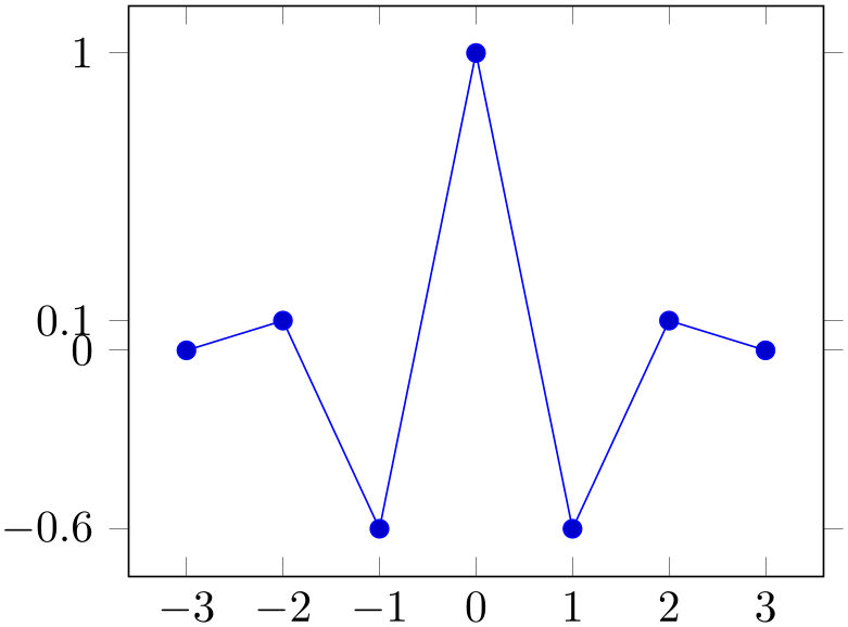
Allows to change the location of the ticks relative to the axis lines. The tick align sets all of them to the same value. Default is “inside”.

% Preamble: \pgfplotsset{width=7cm,compat=1.18}
\begin{tikzpicture}
\begin{axis}[
xtick=data,ytick=data,
xtick align=center,
]
                        \addplot coordinates
                    {
(-3,0) (-2,0.1) (-1,-0.6)
(0,1)
(1,-0.6) (2,0.1) (3,0)
};
\end{axis}
\end{tikzpicture}
% Preamble: \pgfplotsset{width=7cm,compat=1.18}
\begin{tikzpicture}
\begin{axis}[
xtick=data,ytick=data,
ytick align=outside,
]
                        \addplot coordinates
                    {
(-3,0) (-2,0.1) (-1,-0.6)
(0,1)
(1,-0.6) (2,0.1) (3,0)
};
\end{axis}
\end{tikzpicture}
These tick alignment options are set automatically by the axis x line and axis y line methods (unless one appends an asterisk ‘*’):
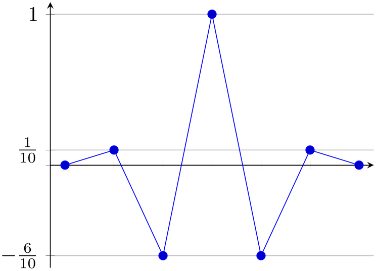
% Preamble: \pgfplotsset{width=7cm,compat=1.18}
\begin{tikzpicture}
\begin{axis}[
xtick=data,
axis x line=center,
xticklabels={,,},
ytick={-0.6,0,0.1,1},
yticklabels={
$-\frac{6}{10}$,,
$\frac{1}{10}$,$1$},
ymajorgrids,
axis y line=left,
enlargelimits=0.05
]
\addplot coordinates
{
(-3,0) (-2,0.1) (-1,-0.6)
(0,1)
(1,-0.6) (2,0.1) (3,0)
};
\end{axis}
\end{tikzpicture}
-
/pgfplots/xticklabel shift={
 dimension
 } (initially empty)
-
/pgfplots/yticklabel shift={
 dimension
 } (initially empty)
-
/pgfplots/zticklabel shift={
 dimension
 } (initially empty)
-
/pgfplots/ticklabel shift={
 dimension
 } (initially empty)
Shifts tick labels in
direction of the outer unit normal of the axis by an amount of
 dimension
 . The ticklabel shift sets the same value for
all axes.
This is usually unnecessary as the anchor of a tick label already yields enough spacing in most cases.
See also axis line shift.
-
/pgfplots/typeset ticklabels with strut(no value) 
-
/pgfplots/default typeset ticklabel(no value) 
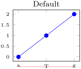
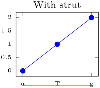
Typically, pgfplots typesets ticks “as is”. This works good in almost all cases, especially if you just have numbers as tick labels.
But it needs adoptions if one ticklabel has text below the baseline and one does not. It is purpose of typeset ticklabels with strut to align them.
% Preamble: \pgfplotsset{width=7cm,compat=1.18}
\begin{tikzpicture}
\begin{axis}[
title=Default,
tiny,
symbolic x coords={a,T,g},
xticklabel style={name=tick no \ticknum},
xtick=data,
]
\addplot coordinates {(a,0) (T,1) (g,2)};
\end{axis}
\draw [red,opacity=0.5]
                            (tick no 0.base) --
                    (tick no 2.base);
\end{tikzpicture}
\begin{tikzpicture}
\begin{axis}[
title=With strut,
tiny,
symbolic x coords={a,T,g},
xtick=data,
xticklabel style={name=tick no \ticknum},
typeset ticklabels with strut,
]
\addplot coordinates {(a,0) (T,1) (g,2)};
\end{axis}
\draw [red,opacity=0.5]
                            (tick no 0.base) --
                    (tick no 2.base);
\end{tikzpicture}
In order to make the normalize the tick labels, pgfplots automatically inserts \strut. A \strut is a TeX macro which inserts an empty box of “full height”, including anything above or below the text’s baseline.
For standard axes, this key is basically equivalent to xticklabel=\strut\pgfmathprintnumber{\tick}.
Note that \strut is off by default as enlarges the bounding box unnecessarily for pure numeric nodes. This is particularly unexpected for polaraxis, but also for normal plots.
4.15.3Tick Scaling – Common Factors In Ticks
-
/pgfplots/scaled ticks=true|false|base 10:
 e
e |real:
 num
num |manual:{
 label
label }{
}{ code
code } (initially true)
-
/pgfplots/scaled x ticks=
 one of the values
 (initially true)
-
/pgfplots/scaled y ticks=
 one of the values
 (initially true)
-
/pgfplots/scaled z ticks=
 one of the values
 (initially true)
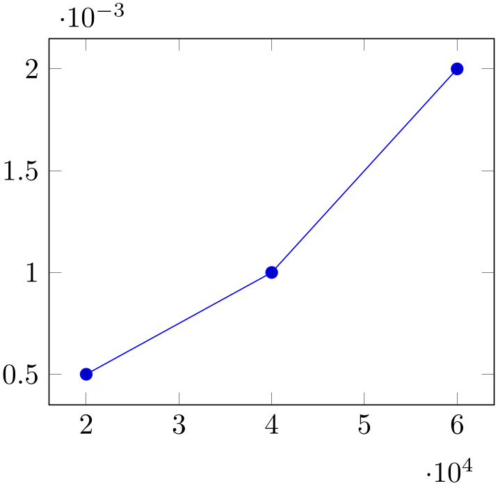
Allows to factor out common exponents in tick labels for linear axes. For example, if you have tick labels \(20000,40000\) and \(60000\), you may want to save some space and write \(2,4,6\) with a separate factor ‘\(\cdot 10^4\)’. Use ‘scaled ticks=true’ to enable this feature. In case of true, tick scaling will be triggered if the data range is either too large or too small (see below).
% Preamble: \pgfplotsset{width=7cm,compat=1.18}
\begin{tikzpicture}
\begin{axis}[scaled ticks=true]
                        \addplot coordinates
                    {
(20000,0.0005)
(40000,0.0010)
(60000,0.0020)
};
\end{axis}
\end{tikzpicture}%
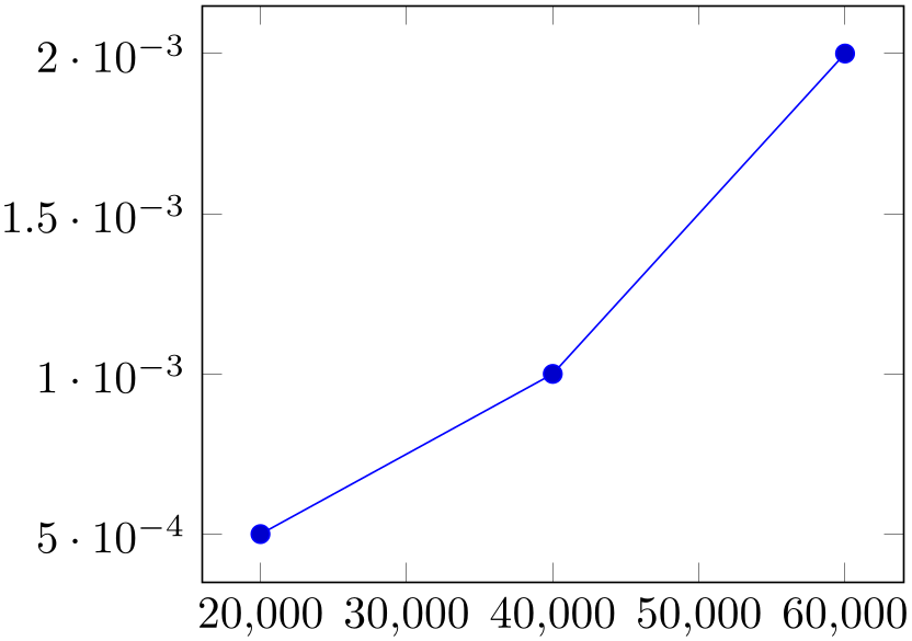
% Preamble: \pgfplotsset{width=7cm,compat=1.18}
\begin{tikzpicture}
\begin{axis}[
scaled ticks=false,
]
                        \addplot coordinates
                    {
(20000,0.0005)
(40000,0.0010)
(60000,0.0020)
};
\end{axis}
\end{tikzpicture}
The scaled ticks key is a style which simply sets scaled ticks for both, \(x\) and \(y\).
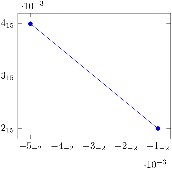
The value base 10: e
e allows to adjust the algorithm manually. For example, base 10:3 will divide every tick label by \(10^3\):
% Preamble: \pgfplotsset{width=7cm,compat=1.18}
\begin{tikzpicture}
\begin{axis}[
scaled ticks=base 10:3,
/pgf/number format/sci subscript,
]
                        \addplot coordinates
                    {
(-0.00001,2e12) (-0.00005,4e12)
};
\end{axis}
\end{tikzpicture}
Here, the sci subscript option simply saves space. In general, base 10:\(e\) will divide every tick by \(10^e\). The effect is not limited by the “too large or too small” decisions mentioned above.
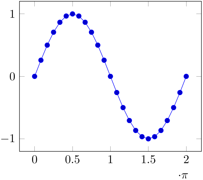
The value real: num
num allows to divide every tick by a fixed
 num
num . For example, the following plot is physically ranged from \(0\) to \(2\pi \), but the tick scaling algorithm is
configured to divide every tick label by \(\pi \).
% Preamble: \pgfplotsset{width=7cm,compat=1.18}
\begin{tikzpicture}
\begin{axis}[
xtick={0,1.5708,...,10},
domain=0:2*pi,
scaled x ticks={real:3.1415},
xtick scale label code/.code={$\cdot \pi$},
]
\addplot {sin(deg(x))};
\end{axis}
\end{tikzpicture}
Setting scaled ticks=real: num
num also changes the
tick scale label code to
\pgfkeys{/pgfplots/xtick scale label code/.code=
{$\pgfkeysvalueof{/pgfplots/tick scale binop} \pgfmathprintnumber{#1}$},
}
The key tick scale binop is described below, it is set initially to \cdot.
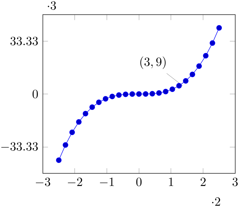
A further – not very useful – example is shown below. Every \(x\) tick label has been divided by \(2\), every \(y\) tick label by \(3\).
% Preamble: \pgfplotsset{width=7cm,compat=1.18}
\begin{tikzpicture}
\begin{axis}[
scaled x ticks=real:2,
scaled y ticks=real:3,
]
\addplot {x^3};
                        \node [pin=135:{$(3,9)$}] at
                    (3,9) {};
\end{axis}
\end{tikzpicture}
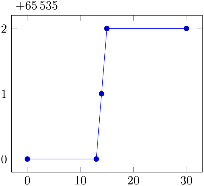
The last option, scaled ticks=manual:{ label
label }{
}{ code
code } allows even more customization. It allows full control over the displayed scaling label and the scaling
code:
 label
label is used as is inside of the tick scaling label while
 code
code is supposed to be a one argument macro which scales each tick. Example:
% Preamble: \pgfplotsset{width=7cm,compat=1.18}
\begin{tikzpicture}
\begin{axis}[
scaled y ticks=manual:{$+65\,535$}{
\pgfmathparse{#1-65535}
},
yticklabel style={
/pgf/number format/fixed,
/pgf/number format/precision=1,
},
]
                        \addplot coordinates
                    {
(0, 65535)
(13, 65535)
(14, 65536)
(15, 65537)
(30, 65537)
};
\end{axis}
\end{tikzpicture}
The example uses $+65\,535$ as tick scale label content. Furthermore, it defines the customized tick label formula \(y - (+6.5535\cdot 10^4) = y - 65535\) to generate \(y\) tick labels.
The
 label
label can be arbitrary. It is completely in user control. The second argument,
 code
code is supposed to be a one-argument-macro in which #1 is the current tick position in floating point representation.
The macro is expected to assign \pgfmathresult (as a
number). The pgf manual [7] contains detailed documentation about its math engine.
This feature may also be used do transform coordinates in case they can’t be processed with pgfplots: transform them and supply a proper tick scaling method such that tick labels represent the original range.
If
 label
label is empty, the tick scale label won’t be drawn (and no space will be occupied).
Tick scaling does not work for logarithmic axes.
Allows to change the default code for scaled tick labels. The default is
More precisely, it is
\pgfplotsset{
xtick scale label code/.code={$\pgfkeysvalueof{/pgfplots/tick scale binop} 10^{#1}$},
}
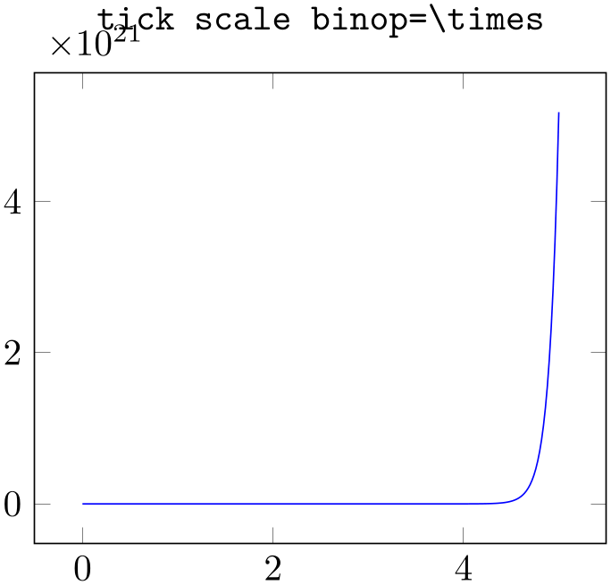
and the initial value of tick scale binop is \cdot, but it can be changed to \times if desired.
If the code is empty, no tick scale label will be drawn (and no space is consumed).
A style which sets xtick scale label code and those for \(y\) and \(z\).
-
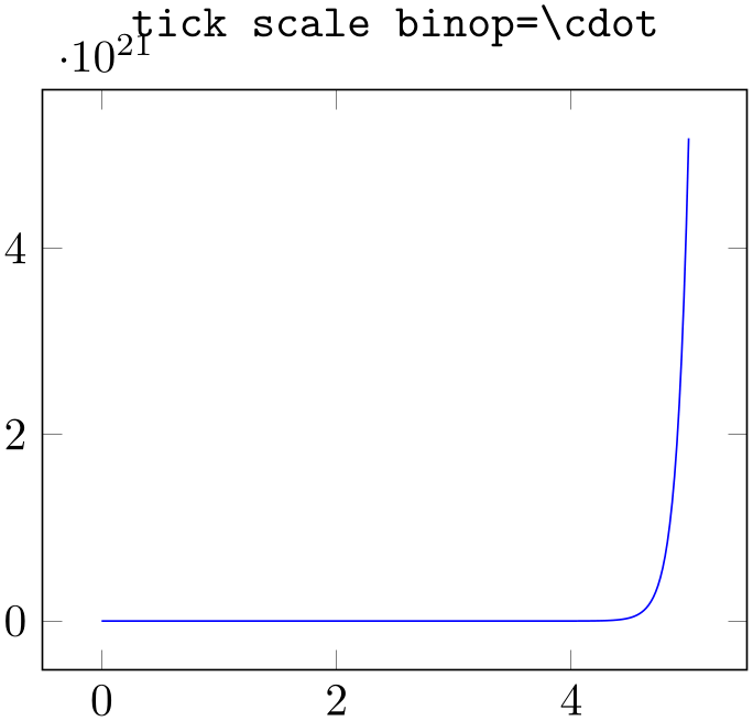
/pgfplots/tick scale binop={
 TeX
math operator
 } (initially \cdot)
Sets the binary operator used to display tick scale labels.
% Preamble: \pgfplotsset{width=7cm,compat=1.18}
\begin{tikzpicture}
\begin{axis}[
title=\texttt{tick scale
binop=\textbackslash cdot},
]
\addplot [
mark=none,
blue,
samples=250,
domain=0:5,
] {exp(10*x)};
\end{axis}
\end{tikzpicture}
% Preamble: \pgfplotsset{width=7cm,compat=1.18}
\begin{tikzpicture}
\begin{axis}[
title=\texttt{tick scale
binop=\textbackslash times},
tick scale binop=\times,
]
\addplot [
mark=none,
blue,
samples=250,
domain=0:5,
] {exp(10*x)};
\end{axis}
\end{tikzpicture}
-
/pgfplots/scale ticks below exponent={
 exponent
 } (initially -1)
Allows fine tuning of the ‘scaled ticks’ algorithm: if the axis limits are of magnitude \(10^e\) and \(e<\) exponent
 , the common prefactor \(10^e\) will be factored out. The default is
-
/pgfplots/scale ticks above exponent={
 exponent
 } (initially 3)
Allows fine tuning of the ’scaled ticks’ algorithm: if the axis limits are of magnitude \(10^e\) and \(e>\) exponent
 , the common prefactor \(10^e\) will be factored out.
4.15.4Tick Fine-Tuning
The tick placement algorithm depends on a number of parameters which can be tuned to get better results.
-
/pgfplots/try min ticks={
 number
 } (initially 4)
Configures a loose lower bound on the number of ticks. It should be considered as a suggestion, not a tight limit. This number will increase the number of ticks if ‘max space between ticks’ produces too few of them.
The total number of ticks may still vary because not all fractional numbers in the axis’ range are valid tick positions.
-
/pgfplots/try min ticks log={
 number
 } (initially 3)
The same as try min ticks, but for logarithmic axis.
-
/pgfplots/tickwidth={
 dimension
 } (initially 0.15cm)
-
/pgfplots/major tick length={
 dimension
 } (initially 0.15cm)
Sets the length of major tick lines.
It can be accessed using \pgfkeysvalueof{/pgfplots/major tick length}.
-
/pgfplots/subtickwidth={
 dimension
 } (initially 0.1cm)
-
/pgfplots/minor tick length={
 dimension
 } (initially 0.1cm)
Sets the length of minor tick lines.
It can be accessed using \pgfkeysvalueof{/pgfplots/minor tick length}.
-
/pgfplots/xtick placement tolerance(initially 0.05pt) 
-
/pgfplots/ytick placement tolerance(initially 0.05pt) 
-
/pgfplots/ztick placement tolerance(initially 0.05pt) 
Tick lines and labels will be placed if they are no more than this tolerance beyond the axis limits. This threshold should be chosen such that it does not produce visible differences while still providing fault tolerance.
The threshold is given in paper units of the final figure.
-
/pgfplots/log basis x={
 number
 } (initially empty)
-
/pgfplots/log basis y={
 number
 } (initially empty)
-
/pgfplots/log basis z={
 number
 } (initially empty)
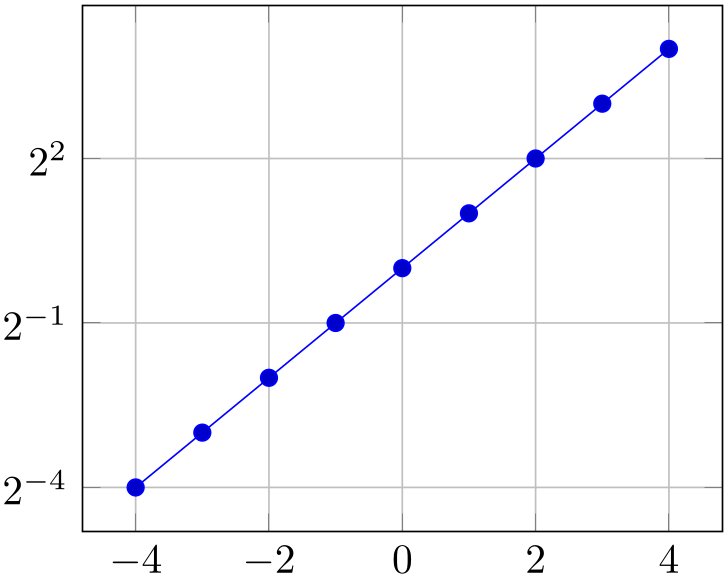
Allows to change the logarithms used for logarithmic axes.
Changing to a different log basis is nothing but a scale. However, it also changes the way tick labels are displayed: they will also be shown in the new basis.
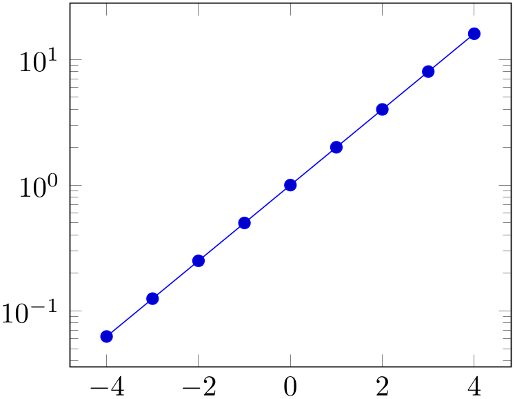
% Preamble: \pgfplotsset{width=7cm,compat=1.18}
\begin{tikzpicture}
\begin{semilogyaxis}[log basis y=2,grid=major,samples at={-4,...,4}]
\addplot {2^x};
\end{semilogyaxis}
\end{tikzpicture}
~
\begin{tikzpicture}
\begin{semilogyaxis}[log basis y=10,samples at={-4,...,4}]
\addplot {2^x};
\end{semilogyaxis}
\end{tikzpicture}
The initial setting is ‘log basis x=’ which defaults to: the natural logarithm for any coordinates (basis \(\exp (1)\)), and the logarithm base \(10\) for the display of tick labels.
If the log basis is changed to something different than the empty string, the chosen logarithm will be applied to any input coordinate (if the axis scale is log as well) and tick labels will be displayed in this basis.
In other words: usually, you see log-axes base \(10\) and that’s it. It is only interesting for coordinate filters:
the initial setting (with empty
 number
 ) uses coordinate lists basis \(e\) although the display will use basis \(10\) (i.e. it is rescaled). Any non-empty
value
 number
 causes both, coordinate lists and display to use
 number
 as basis for the logarithm. The JavaScript code of the
clickable library will always use the display basis (which
is usually \(10\)) when it computes slopes.
Please note that xtickten will be used differently now: it will provide the desired ticks in the new basis! Despite the misleading name “ten”, xtickten={1,2,3,4} will yield ticks at \(2^1,2^2,2^3,2^4\) if log basis x=2 has been set.
-
/pgfplots/hide obscured x ticks=true|false (initially true) 
-
/pgfplots/hide obscured y ticks=true|false (initially true) 
-
/pgfplots/hide obscured z ticks=true|false (initially true) 
Allows to configure whether pgfplots should hide ticks and their labels if it assumes that they are obscured by other axis lines.
% Preamble: \pgfplotsset{width=7cm,compat=1.18}
\begin{tikzpicture}
\begin{axis}[
footnotesize,
axis x line=center,
axis y line=center,
% hide obscured x ticks=false,
% hide obscured y ticks=false,
]
\addplot {x};
\end{axis}
\end{tikzpicture}
% Preamble: \pgfplotsset{width=7cm,compat=1.18}
\begin{tikzpicture}
\begin{axis}[
footnotesize,
axis x line=center,
axis y line=center,
hide obscured x ticks=false,
hide obscured y ticks=false,
]
\addplot {x};
\end{axis}
\end{tikzpicture}
Note that this key applies if only and only if one of axis x line, axis y line, or axis z line is not box.