Manual for Package pgfplots
2D/3D Plots in LATeX, Version 1.18.1
http://sourceforge.net/projects/pgfplots

/pgfplots/x filter/.expression={math expression} ¶

/pgfplots/y filter/.expression={math expression} ¶

/pgfplots/z filter/.expression={math expression} ¶

Installs a coordinate filter which allows to modify the current value of a single coordinate.

The argument math expression is a math expression which contains x, y, or z.



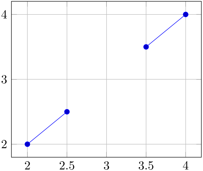
copy % Preamble: \pgfplotsset{width=7cm,compat=1.18} \begin{tikzpicture} \begin{axis}[grid=major] \addplot+ [ unbounded coords=jump, x filter/.expression={x+1}, y filter/.expression={y==3 ? nan : y}, ] table { x y 1 2 1.5 2.5 2 3 2.5 3.5 3 4 }; \end{axis} \end{tikzpicture}

The x filter is evaluated first. It can depend on x, y, and z whose values are the “prepared” coordinates: values which have been found after applying x coord trafo and any logarithms (for logarithmic axes).

The y filter is evaluated as next. It can depend on x which is the result of x filter. It can also depend on y and z which have the same value as discussed in the previous paragraph.

The z filter is evaluated as last. It can depend on x and y which are result of their respective filters. It can also depend on z which is the plain \(z\)-coordinate (as discussed for x filter).

Note that filter values can contain expandable material, including \thisrow for tables:



copy % Preamble: \pgfplotsset{width=7cm,compat=1.18} \begin{tikzpicture} \begin{axis} \addplot+[ x filter/.expression={ \thisrow{W} == 42 ? 0.2 : x }, ] table { x y W 0 0 41 0.5 0.5 42 1 1 43 }; \end{axis} \end{tikzpicture}

Defining filters by math expression is actually a special case of x filter, see below. As a consequence, the expression may contain \pgfmathresult which is the unmodified input value (see the specification of x filter below).

/pgfplots/x filter/.append expression={math expression}

/pgfplots/y filter/.append expression={math expression}

/pgfplots/z filter/.append expression={math expression}

These are variants of x filter/.expression which allow to append another coordinate filter. In this case, you can have different filters for the same coordinate, and each is based on the output of the previous filter:



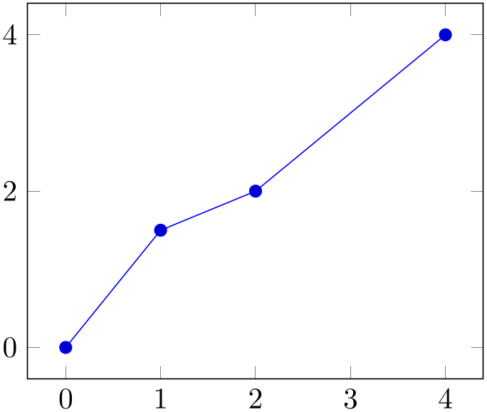
copy % Preamble: \pgfplotsset{width=7cm,compat=1.18} \begin{tikzpicture} \begin{axis} \addplot+[ y filter/.append expression={ abs(x-1) < 1e-4 ? 1.5 : \pgfmathresult }, y filter/.append expression={ abs(x-3) < 1e-4 ? NaN : \pgfmathresult }, ] table { x y 0 0 1 1 2 2 3 3 4 4 }; \end{axis} \end{tikzpicture}

The example installs two y filters: the first checks if \(x = 1\) and defines \(y=1.5\) in this case, otherwise it tells the filter to “use the value of \(y\) as it was before the filter”. The second filter checks if \(x = 3\) and assigns the value “Not a Number” if that is the case (which discards the coordinate). Otherwise it tells the filter to “use the value of \(y\) as it was before the filter”, which is the value generated by the first filter.

As you see, the special macro “\pgfmathresult” always yields the unmodified input value. This is a property of the underlying x filter functionality.

Note that the example could be rephrased by replacing the first “\pgfmathresult” by “y”. But in order to simplify copy/paste, it makes sense to formulate incremental filters in a way which is always incremental.

Installing x filter/.append expression is the same as x filter/.expression if there was no other filter in place beforehand. The “append” functionality is applied even if there is some customized x filter in place (for example one installed with x filter/.code as outlined below). Thus, “append” has the semantics “append a further coordinate filter” rather than “append another expression to an existing expression”. The only requirement is that a previous filter must not replace a coordinate by an empty value. Filters which silently discard the value and return an empty one must be appended after .append expression.

/pgfplots/x filter/.code={...} ¶

/pgfplots/y filter/.code={...} ¶

/pgfplots/z filter/.code={...} ¶

/pgfplots/filter point/.code={...} ¶

The code keys x filter and y filter are advanced variants of x filter/.expression and its variants. They allow to modify single coordinate values, but can execute arbitrary TeX code. A coordinate filter gets an input coordinate as #1 (on input, the same value is stored in \pgfmathresult), applies some operation and writes the result into the macro \pgfmathresult. If \pgfmathresult is empty afterwards, the coordinate is discarded. You can also set \pgfmathresult to nan or inf in which case the coordinate can be either discarded (if unbounded coords=discard is set) or the plot can be interrupted (the case unbounded coords=jump).

The filter point/.code filter allows filtering depending on all components forming a complete point (\(x\), \(y\) and \(z\)); it is described below.

It is allowed that filters do not change \pgfmathresult. In this case, the unfiltered coordinate will be used.

Coordinate filters are useful in automatic processing system, where pgfplots is used to display automatically generated plots. You may not want to filter your coordinates by hand, so these options provide a tool to do this automatically.

The following filter adds \(0.5\) to every \(x\)-coordinate.



copy % Preamble: \pgfplotsset{width=7cm,compat=1.18} \begin{tikzpicture} \begin{axis}[ % equivalent to 'x filter/.expression={x+0.5}' x filter/.code={ \pgfmathadd{#1}{0.5}, }, ] \addplot coordinates { (4,0) (6,1) }; \end{axis} \end{tikzpicture}

Please refer to [7, pgfmath manual] for details about the math engine of pgf. Whenever possible, math-based filters should be formulated using x filter/.expression as that reduces the complexity and ensures the best precision (it also works with lua backend).

During evaluation of the filter, the macro \coordindex contains the number of the current coordinate (starting with \(0\)). Thus, the following filter discards all coordinates after the \(5\)th and before the \(10\)th.



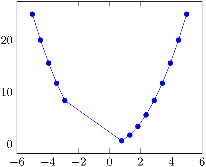
copy % Preamble: \pgfplotsset{width=7cm,compat=1.18} \begin{tikzpicture} \begin{axis}[ samples=20, % equivalent to % x filter/.expression={ % \coordindex>4 && \coordindex<11 ? nan : x % }, x filter/.code={ \ifnum\coordindex>4 \ifnum\coordindex<11 \def\pgfmathresult{} \fi \fi }, ] \addplot {x^2}; \end{axis} \end{tikzpicture}

There is also a style key which simplifies selection by index, see below.

pgfplots invokes the filter with argument #1 set to the input coordinate. For \(x\) filters, this is the \(x\)-coordinate as it is specified to \addplot, for \(y\) filters it is the \(y\)-coordinate.

If the corresponding axis is logarithmic, #1 is the logarithm (see log basis x and its variants) of the coordinate as a real number, for example #1=4.2341. In case the logarithm was undefined, the argument will be empty.

The arguments to coordinate filters are minimally preprocessed: first, for logarithmic axes, the log of the argument is supplied. Second, any high level coordinate maps like x coord trafo (which may be used to map dates to numbers or string to numbers or so) are applied. In consequence, the #1 argument is supposed to be a number. No further transformation has been applied.

Occasionally, it might be handy to get the “raw”, completely unprocessed input coordinate as it has been reported by the coordinate input routine. This unprocessed data is available in the three math parser constants rawx, rawy and rawz. All these values are ready for use in filters (and some other methods influence plots as well). Note that rawy is to be used like a function without arguments, i.e. filters can employ it where math parsing is done.

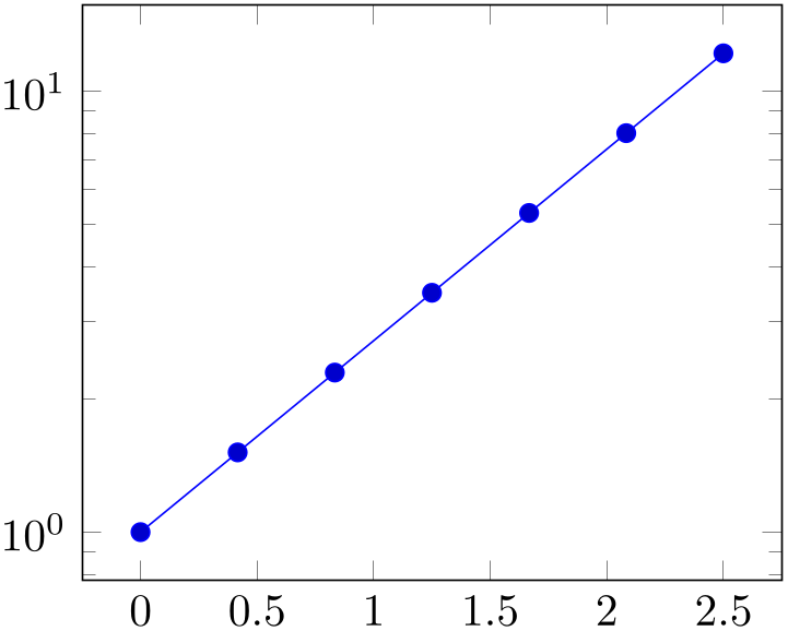
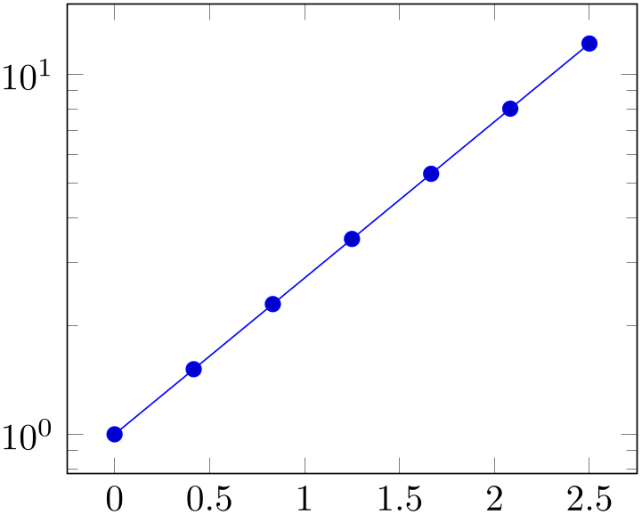
An application could be to filter log values based on the normal scale:



copy % Preamble: \pgfplotsset{width=7cm,compat=1.18} \begin{tikzpicture} \begin{semilogyaxis} \addplot+ [ restrict expr to domain={rawy}{1e0:1.5e1}, ] {exp(x)}; \end{semilogyaxis} \end{tikzpicture}

The preceding example uses rawy to throw all samples outside of the range \([1,15]\) away.

If key filters are invoked for \addplot table, access to the current row’s data can be achieved using \thisrow{column name} (and its variants). This includes all columns of the table.

The filter point key is more technical. It doesn’t take an argument: its arguments are given in terms of the pgfkeys variables /data point/x, /data point/y and /data point/z. It may change its coordinates using \pgfkeyssetvalue{/data point/x}{new value}; access to variables can be achieved with \pgfkeysvalueof{/data point/x} or, if the argument shall be written into a macro, with \pgfkeysgetvalue. This filter is evaluated after the other ones.

Note that you can provide different x filter/y filter arguments to each \addplot command. It seems there are only problems with the ‘#1’ argument, and I haven’t yet found out why. Please use \pgfmathresult in place of #1 if you provide \addplot[x filter/.code={...}].

Note that coordinate filtering is also available for mesh, surf, and patch plots. In this context, a patch type is drawn if and only if all its vertices have bounded coordinates. In other words: if one vertex of, say, a rectangle has been filtered away, the entire rectangle will be omitted. Coordinate filtering for mesh and surface plots has a further special requirement: the default for such plots is mesh input=lattice. If a coordinate filter silently discards a coordinate, the lattice will break and pgfplots will become confused. Consequently, coordinate filtering for mesh and surface plots always needs unbounded coords=jump, and any point which is filtered away should receive the value nan instead of an empty string (since empty strings will always be discarded even in presence of unbounded coords=jump). Please see the reference documentation of unbounded coords and the example therein on page (page for section 4.5.14) for details about coordinate filtering and three dimensional plots.

/pgfplots/pre filter/.code={...} ¶

Applied before x filter, y filter, and z filter.

/pgfplots/skip coords between index={begin}{end} ¶

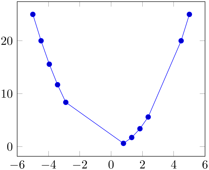
A style which appends an x filter which discards selected coordinates. The selection is done by index where indexing starts with \(0\), see \coordindex. Every coordinate with index \(\meta {begin} \le i < \meta {end}\) will be skipped.



copy % Preamble: \pgfplotsset{width=7cm,compat=1.18} \begin{tikzpicture} \begin{axis}[ samples=20, skip coords between index={5}{11}, skip coords between index={15}{18}, ] \addplot {x^2}; \end{axis} \end{tikzpicture}

Technical note:

this style usually applies to \(x\)-coordinates (i.e. it counts \(x\)-coordinates). In case you want to apply it to something like hist/data or quiver/u, you can

• 1. append an asterisk ‘*’ to the style’s name and

• 2. provide the target coordinate’s name as first argument.

For example, skip coords between index*={hist/data}{2}{4} applies to hist/data.

/pgfplots/each nth point={integer} ¶

A style which appends an x filter which discards all but each \(n\)th input coordinate.

This downsampling works fairly well. It can be used to reduce a huge amount of coordinates from an input file. In this case, you should also set filter discard warning=false to avoid repeated notifications about skipped coordinates and unbounded coords=discard such that pgfplots should silently forget any discarded points (rather than generated interrupted plots).

Note that there is also a mark repeat style which applies the same operation to plot marks only.

Technical note:

this style usually applies to \(x\)-coordinates (i.e. it counts \(x\) coordinates). In case you want to apply it to something like hist/data or quiver/u, you can

• 1. append an asterisk ‘*’ to the style’s name and

• 2. provide the target coordinate’s name as first argument.

For example, each nth point*={hist/data}{2}{4} applies to hist/data.

/pgfplots/restrict x to domain=min:max ¶

/pgfplots/restrict y to domain=min:max ¶

/pgfplots/restrict z to domain=min:max ¶

/pgfplots/restrict x to domain*=min:max ¶

/pgfplots/restrict y to domain*=min:max ¶

/pgfplots/restrict z to domain*=min:max ¶

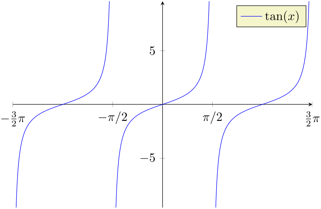
These keys append \(x\) (or \(y\) or \(z\)) coordinate filters to restrict the respective coordinate to a domain.

The versions without star (like restrict x to domain) will assign the value -inf if the coordinate is below min and +inf if the coordinate is above max. The starred versions (like restrict x to domain*) will truncate coordinates to \([\hbox {\meta {min}}, \hbox {\meta {max}}]\), i.e. they assign the value min if the coordinate falls outside of the lower limit and max if the value falls outside of the upper limit.

For logarithmic axes, min and max are logs of the respective values. A variant which uses the non-logarithmic number might be to use restrict expr to domain={\pgfmathrawx}{min}{max}.

The non-starred versions also set unbounded coords=jump which leads to interrupted plots.



copy % Preamble: \pgfplotsset{width=7cm,compat=1.18} \begin{tikzpicture} \begin{axis}[ restrict y to domain=-10:10, samples=1000, % some fine-tuning for the display: width=10cm, height=210pt, xmin=-4.7124, xmax=4.7124, xtick={-4.7124,-1.5708,...,10}, xticklabels={$-\frac32 \pi$,$-\pi/2$,$\pi/2$,$\frac32 \pi$}, axis x line=center, axis y line=center, ] \addplot [blue] gnuplot [id=tangens,domain=-1.5*pi:1.5*pi] {tan(x)}; \legend{$\tan(x)$} \end{axis} \end{tikzpicture}

/pgfplots/restrict expr to domain={expression}{min:max} ¶

/pgfplots/restrict expr to domain*={expression}{min:max} ¶

Appends an \(x\)-coordinate filter which sets the \(x\)-coordinate to -inf if the expression evaluates to something less than min and to inf if expression evaluates to something larger than max.

The starred variant, restrict to domain* assigns min if expression is less then the lower limit and max if it is larger than the upper limit.

The non-starred version also sets unbounded coords=jump which leads to interrupted plots.

In contrast to restrict x to domain, expression can depend on anything which is valid during \addplot, in particular \coordindex or table columns (\thisrow{column name} and friends). The expression doesn’t need to depend on \(x\) at all.

/pgfplots/@restrict to domain={filter name}{expression}{min:max}0|1 ¶

A low-level (technical) key which allows to apply the restrict * to ... features also to something like hist/data.

For example, @restrict to domain={hist/data}{}{0:1}{0} applies the domain-restriction to the histogram-input hist/data. The final ‘0’ means that it works in a similar way as the key restrict x to domain=0:1, i.e. it skips everything which is outside of \([0,1]\). In a similar way, @restrict to domain={hist/data}{}{0:1}{1} applies the functionality of restrict x to domain*=0:1 to hist/data: it truncates values outside of \([0,1]\) to the domain’s end-points.

The filter name is expected to be a coordinate name like x, y, z (or hist/data).

The expression configures an expression which will be used rather than the value of filter name. It can be empty.

The min:max are as described above.

If the last argument is 1, any coordinate outside of the allowed domain will take the domain boundary as value. If it is 0, such a coordinate will get either inf or -inf.

/pgfplots/filter discard warning=true|false (initially true) ¶

Issues a notification in your logfile whenever coordinate filters discard coordinates.