Manual for Package pgfplots
2D/3D Plots in LATeX, Version 1.18.1
http://sourceforge.net/projects/pgfplots

\usepgfplotslibrary{statistics} % LaTeX and plain TeX ¶

\usepgfplotslibrary[statistics] % ConTeXt ¶

\usetikzlibrary{pgfplots.statistics} % LaTeX and plain TeX ¶

\usetikzlibrary[pgfplots.statistics] % ConTeXt ¶

A library which provides plot handlers for statistics.

/pgfplots/boxplot prepared={options with boxplot/ prefix} ¶

\addplot+[boxplot prepared={options with boxplot/ prefix}]

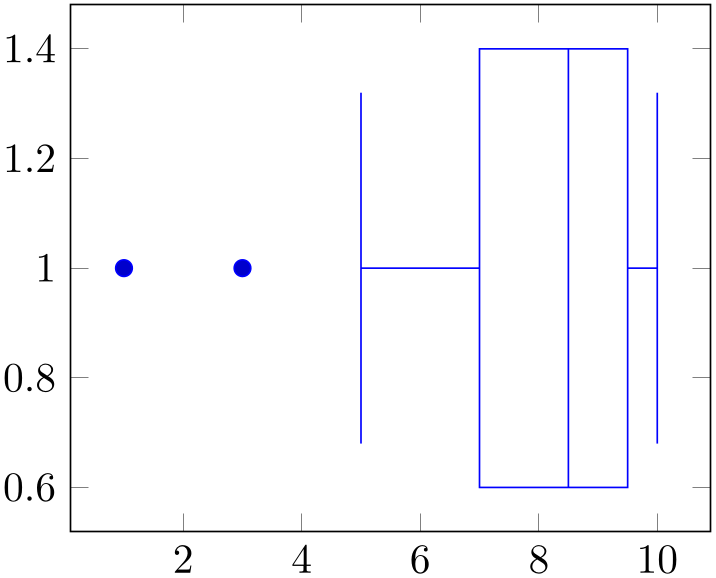
A boxplot prepared takes a couple of key–value pairs which describe the required statistics and a coordinate stream of outliers on input and draws a box plot.



copy % Preamble: \pgfplotsset{width=7cm,compat=1.18}\usepgfplotslibrary{statistics} \begin{tikzpicture} \begin{axis} \addplot+ [ boxplot prepared={ lower whisker=5, lower quartile=7, median=8.5, upper quartile=9.5, upper whisker=10, }, ] table [row sep=\\,y index=0] { data\\ 1\\ 3\\ }; \end{axis} \end{tikzpicture}

The previous example shows the main idea of boxplot prepared: each required quantity has to be provided explicitly using a key–value syntax. The following coordinate stream can be empty; all coordinates inside of it are considered to be outliers. They are drawn as scatter plot.

A box plot produces two coordinates: one which belongs to the input data (for example median) and one which is only used for drawing purposes. Limits will be updated for both of them. While this is clear for the axis which shows the input data (\(x\) in this example, see also draw direction), it should be noted that limits and scaling parameters for the other axis will be chosen just as for any other plot. The box’s extend is a little bit less than one unit by default (compare box extend). As a consequence, one might need to adjust either the limits or the scaling parameters for the remaining axis:



copy % Preamble: \pgfplotsset{width=7cm,compat=1.18}\usepgfplotslibrary{statistics} \begin{tikzpicture} \begin{axis}[ y=1.5cm, ] \addplot+ [ boxplot prepared={ lower whisker=5, lower quartile=7, median=8.5, upper quartile=9.5, upper whisker=10, }, ] table [row sep=\\,y index=0] { data\\ 1\\ 3\\ }; \end{axis} \end{tikzpicture}

/pgfplots/boxplot/draw position={axis unit to place box} (initially 1+\plotnumofactualtype) ¶

The draw position key determines how to choose the position of the box plot, i.e. the axis unit which is free to choose.

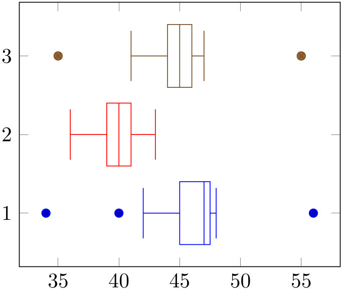
The initial configuration places the first box plot at \(y=1\) and all following ones at the next integer numbers.



copy % Preamble: \pgfplotsset{width=7cm,compat=1.18}\usepgfplotslibrary{statistics} \begin{tikzpicture} \begin{axis} \addplot+ [ boxplot prepared={ lower whisker=42, lower quartile=45, median=47, upper quartile=47.5, upper whisker=48, }, ] table [row sep=\\,y index=0] { 40\\ 34\\ 56\\ }; \addplot+ [ boxplot prepared={ lower whisker=36, lower quartile=39, median=40, upper quartile=41, upper whisker=43, }, ] % no outliers: coordinates {}; \addplot+ [ boxplot prepared={ lower whisker=41, lower quartile=44, median=45, upper quartile=46, upper whisker=47, }, ] coordinates {(0,35) (0,55)}; \end{axis} \end{tikzpicture}

The preceding example shows three box plots in the same axis. Note that they have been aligned using the default setting.

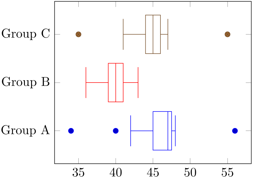
The fact that the first \(N\) boxplot (or the equivalent boxplot prepared) are placed at the coordinates \(1,2,3, \dotsc ,N\) makes it simple to assign tick labels: either use ytick=data or ytick=1,2,3 combined with yticklabels:



copy % Preamble: \pgfplotsset{width=7cm,compat=1.18}\usepgfplotslibrary{statistics} \begin{tikzpicture} \begin{axis}[ ytick={1,2,3}, yticklabels={Group A, Group B, Group C}, ] \addplot+ [ boxplot prepared={ lower whisker=42, lower quartile=45, median=47, upper quartile=47.5, upper whisker=48, }, ] table [row sep=\\,y index=0] { 40\\ 34\\ 56\\ }; \addplot+[ boxplot prepared={ lower whisker=36, lower quartile=39, median=40, upper quartile=41, upper whisker=43, }, ] coordinates {}; \addplot+[ boxplot prepared={ lower whisker=41, lower quartile=44, median=45, upper quartile=46, upper whisker=47, }, ] coordinates {(0,35) (0,55)}; \end{axis} \end{tikzpicture}

The draw position may be read from some input table using draw position=\thisrowcolname. In this case, the last encountered data row will be used (this remark is, of course, only useful if a data stream is present).

While the default choice of draw position hopefully covers the most common use cases, one can also assign a custom value to it if specific box plots should be placed individually:



copy % Preamble: \pgfplotsset{width=7cm,compat=1.18}\usepgfplotslibrary{statistics} \begin{tikzpicture} \begin{axis}[ boxplot/draw direction=y, ] \addplot+ [boxplot prepared={ lower whisker=2.5, lower quartile=4, median=8.5, upper quartile=12, upper whisker=15}, ] coordinates {}; \addplot+ [boxplot prepared={ lower whisker=2.5, lower quartile=4, median=8.5, upper quartile=12, upper whisker=15}, ] coordinates {}; \addplot+ [boxplot prepared={draw position=5, lower whisker=2.5, lower quartile=4, median=8.5, upper quartile=12, upper whisker=15}, ] coordinates {}; \end{axis} \end{tikzpicture}

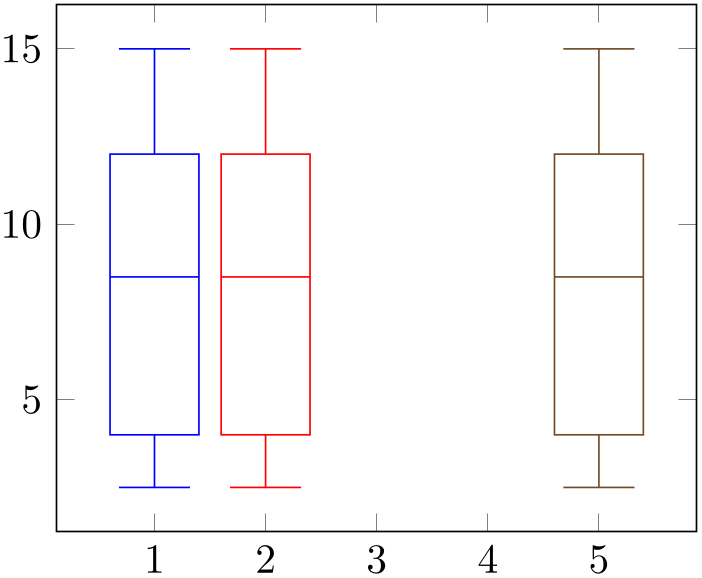
The example shows the first two plots using the default draw position. As this uses the plot index \(+1\), they are placed at \(x=1\) and \(x=2\), respectively (using \(x\) due to draw direction=y). The third plot has draw position=5 and is drawn at \(x=5\).

Note that if you assign draw position for one plot, you may also need to adopt all followings ones as pgfplots does not automatically detect collisions.

/pgfplots/boxplot/data={expression} (initially y) ¶

Tells boxplot how to get its data. The common idea is to provide a mathematical expression which depends on data supplied by the \addplot statement. For example, if you have \addplot expression, the expression may depend upon x, y or z. In case of an \addplot table input routine, the expression can employ \thisrow{colname} to access the currently active table row in the designated column.

It is also possible to avoid invocations of the math parser. Use boxplot/data value={value} instead to do so. Here, value should be of a numeric constant.

The initial configuration employs what would usually become the final y coordinate as input (to be more precise, the initial value is data value=\pgfkeysvalueof{/data point/y}).

/pgfplots/boxplot/data filter/.code={code} (initially empty) ¶

Allows the user to install a filter. This filter works very similarly to the other filters.



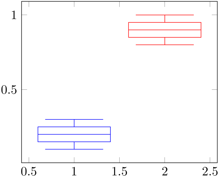
copy % Preamble: \pgfplotsset{width=7cm,compat=1.18}\usepgfplotslibrary{statistics} \pgfplotsset{ only if/.style args={entry of #1 is #2}{ /pgfplots/boxplot/data filter/.code={ \edef\tempa{\thisrow{#1}} \edef\tempb{#2} \ifx\tempa\tempb \else \def\pgfmathresult{} \fi } } } % 'data.dat' contains % v set % 0.1 a % 0.2 a % 0.3 a % 0.8 b % 0.9 b % 1.0 b \begin{tikzpicture} \begin{axis}[ boxplot, table/y=v, boxplot/draw direction=y, ] \addplot table[only if={entry of set is a}]{data.dat}; \addplot table[only if={entry of set is b}]{data.dat}; \end{axis} \end{tikzpicture}

/pgfplots/boxplot/lower whisker={value} (initially auto) ¶

/pgfplots/boxplot/lower quartile={value} (initially auto) ¶

/pgfplots/boxplot/median={value} (initially auto) ¶

/pgfplots/boxplot/upper quartile={value} (initially auto) ¶

/pgfplots/boxplot/upper whisker={value} (initially auto) ¶

/pgfplots/boxplot/average={value} (initially empty) ¶

These keys constitute the supported statistics. Typically, a box plot uses each of them except for average.

Any numeric value for value will be used as is. This holds for both boxplot prepared and boxplot.

An empty value disables the respective key: its associated visualization will be omitted. This is the default for average.

The value auto tells pgfplots to include the statistics in the automatic computation applied by boxplot. It is irrelevant for boxplot prepared (where it is essentially the same as an empty value).

The definition of the values is as follows. Assume that we have a given sample of a distribution, say \(x_1,\dotsc ,x_N\), and assume that the values are sorted, \(x_1 < \dotsb < x_N\) (which is not a requirement for boxplot, by the way). For any real number \(p\) with \(0\le p\le 1\), the “\(p\)-quantile” (or \(p\)–percentage) is defined as

\[ x_p := \begin {cases} x_{N \cdot p} & \text {if $N \cdot p$ is an integer number}\\ \frac {1}{2} (x_{\lfloor N p \rfloor } + x_{\lceil N \cdot p \rceil }) & \text {if $N \cdot p$ is not an integer.} \end {cases} \]

median is the \(0.5\)-quantile of the input data: half of the points are less and half of the points are larger than the median.

lower quartile is the \(0.25\)-quantile of the input data.

upper quartile is the \(0.75\)-quartile of the input data.

lower whisker is the smallest data value which is larger than lower quartile \(-1.5 \cdot \text {IQR}\) where \(\text {IQR}\) is the “interquartile range”, i.e. the difference between upper quartile and lower quartile.

upper whisker is the largest data value which is smaller than upper quartile \(+1.5 \cdot \text {IQR}\).

average is the sample average. It is omitted by boxplot in its default configuration. Set it to auto to enable its auto-computation.

/pgfplots/boxplot/draw direction=x|y (initially x) ¶

Since boxplot is inherently one-dimensional, it can be visualized along the \(x\)- or the \(y\)-axis.

The default configuration uses the \(x\) direction as seen above.

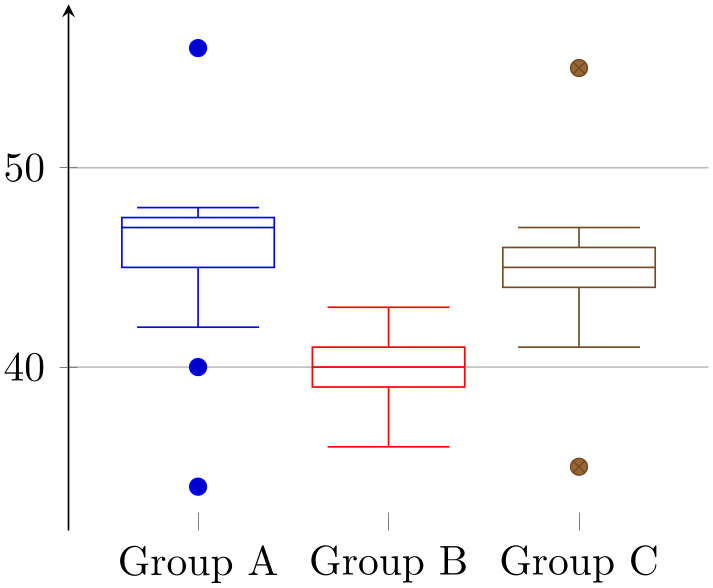
The alternative choice \(y\) lets the boxes and their whiskers extend along the \(y\)-axis and stacks multiple box plots along the \(x\)-axis:



copy % Preamble: \pgfplotsset{width=7cm,compat=1.18}\usepgfplotslibrary{statistics} \begin{tikzpicture} \begin{axis}[ boxplot/draw direction=y, x axis line style={opacity=0}, axis x line*=bottom, axis y line=left, enlarge y limits, ymajorgrids, xtick={1,2,3}, xticklabels={Group A, Group B, Group C}, ] \addplot+ [ boxplot prepared={ lower whisker=42, lower quartile=45, median=47, upper quartile=47.5, upper whisker=48, }, ] table [row sep=\\,y index=0] { 40\\ 34\\ 56\\ }; \addplot+ [ boxplot prepared={ lower whisker=36, lower quartile=39, median=40, upper quartile=41, upper whisker=43, }, ] coordinates {}; \addplot+[ boxplot prepared={ lower whisker=41, lower quartile=44, median=45, upper quartile=46, upper whisker=47, }, ] coordinates {(0,35) (0,55)}; \end{axis} \end{tikzpicture}

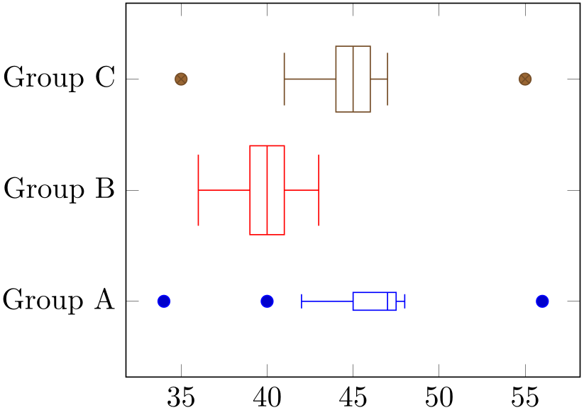
/pgfplots/boxplot/variable width=true|false (initially false) ¶

If enabled, the box extend will be scaled according to the sample size relative to all other boxplot or boxplot prepared within the same axis.

The key variable width only has an effect if sample size is available. For boxplot prepared, one needs to provide sample size explicitly.



copy % Preamble: \pgfplotsset{width=7cm,compat=1.18}\usepgfplotslibrary{statistics} \begin{tikzpicture} \begin{axis}[ ytick={1,2,3}, yticklabels={Group A, Group B, Group C}, boxplot/variable width, ] \addplot+ [% Group A: boxplot prepared={ lower whisker=42, lower quartile=45, median=47, upper quartile=47.5, upper whisker=48, sample size=1000, }, ] table [row sep=\\,y index=0] { 40\\ 34\\ 56\\ }; \addplot+ [% Group B: boxplot prepared={ lower whisker=36, lower quartile=39, median=40, upper quartile=41, upper whisker=43, sample size=100000, }, ] coordinates {}; \addplot+ [% Group C: boxplot prepared={ lower whisker=41, lower quartile=44, median=45, upper quartile=46, upper whisker=47, sample size=50000, }, ] coordinates {(0,35) (0,55)}; \end{axis} \end{tikzpicture}

The variable width computation computes the largest and smallest value of sample size, chosen among all box plots in the same axis. If a single plot has no sample size, it will be omitted from the computation (and it will not be scaled). If a single box plot has variable width=false, its sample size will not contribute either. The box plot with largest value of sample size will be drawn with \(100\%\) of box extend. The box plot with smallest value will be drawn with variable width min target times box extend as size (i.e. it will receive the smallest configured size). All box plots in-between are scaled linearly.

Note that the previous paragraph is not entirely true: sample size is only indirectly related to the scaling factor. Instead, the variable width expr is evaluated with the sample size as argument (see below for details).

/pgfplots/boxplot/sample size={number} (initially auto) ¶

The number of samples used to derive the statistics. This number is used if variable width=true.

The value auto means to “use it whenever it can be acquired somewhere”. For a boxplot, it means that the size of the input sample is taken as is. For a boxplot prepared, it means that the data is unavailable.

The empty string means that the value is unavailable.

Otherwise, a number is expected.

/pgfplots/boxplot/variable width expr={math expression} (initially sqrt(#1)) ¶

A math expression which is used to evaluate the scaling factors of variable width. The argument is the current value of sample size. This key is used to implement common (nonlinear) transformations which are to be applied to the sample size before the result is used to scale down box sizes.

Typically, the argument should be a monotonically increasing function.

/pgfplots/boxplot/sample size min={min sample size of group} (initially empty) ¶

/pgfplots/boxplot/sample size max={max sample size of group} (initially empty) ¶

This is part of the variable width scaling: it is used to determine the box extend relative to all other box plots of the same group. It fixes the range.

/pgfplots/boxplot/variable width min target={factor for the box width minimal size} (initially 0.2) ¶

Used for the variable width feature to determine the size for the box plot with smallest value of sample size. The argument is interpreted to be a scaling factor in the range \([0,1]\).

It is to be understood as percentage of box extend: a value of \(1\) means \(100\%\) of box extend. The initial configuration is 0.2, meaning \(20\%\) of box extend.

The box plot with largest value of sample size has \(100\%\) of box extend.

/pgfplots/boxplot/box extend={axis unit for box extension} (initially 0.8) ¶

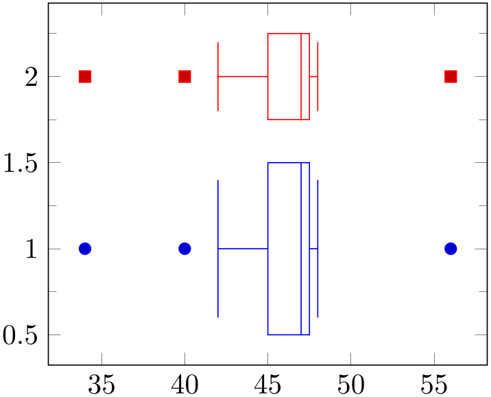
A parameter which controls the size of the boxes with respect to the axis orthogonal to the data axis.

The box extend is used as follows: if a box is centered at say, \(y=1\) with box extend=1, the box will start at \(\nicefrac {1}{2}\) and will end at \(1 \nicefrac {1}{2}\). In other words: the box size is \(1\) \(y\) unit.

It is interpreted as coordinate in the axis, and it affects the automatic computation of ymin and ymax values for a boxplot.



copy % Preamble: \pgfplotsset{width=7cm,compat=1.18}\usepgfplotslibrary{statistics} \begin{tikzpicture} \begin{axis}[minor y tick num=1] \addplot+ [ boxplot prepared={ lower whisker=42, lower quartile=45, median=47, upper quartile=47.5, upper whisker=48, box extend=1, }, ] table [row sep=\\,y index=0] { 40\\ 34\\ 56\\ }; \addplot+ [ boxplot prepared={ lower whisker=42, lower quartile=45, median=47, upper quartile=47.5, upper whisker=48, box extend=0.5, }, ] table [row sep=\\,y index=0] { 40\\ 34\\ 56\\ }; \end{axis} \end{tikzpicture}

The box extend controls the size of the box and the length of the median line. It also controls the size of whiskers, although they have a separate parameter whisker extend.

It is supposed to be the low-level size of a box plot, although it can be interpreted and used as a “low-level variant” of variable width.

/pgfplots/boxplot/whisker extend={axis unit for whisker extension} (initially \pgfkeysvalueof{/pgfplots/boxplot/box extend}*0.8) ¶

A parameter which configures how large whisker lines are with respect to the non-data axis.

It is used in the same way as box extend, and it also affects axis limits.

The initial configuration couples its value to box extend (it is \(80\%\) of box extend, to be more precise).

/pgfplots/boxplot/draw relative anchor={number between \(0\) and \(1\)} (initially 0.5) ¶

A key which customizes the anchor inside of the box where the whiskers are attached.



copy % Preamble: \pgfplotsset{width=7cm,compat=1.18}\usepgfplotslibrary{statistics} \begin{tikzpicture} \begin{axis}[y=1cm] \addplot+ [ boxplot prepared={ lower whisker=42, lower quartile=45, median=47, upper quartile=47.5, upper whisker=48, draw relative anchor=0, }, ] table [row sep=\\,y index=0] { 40\\ 34\\ 56\\ }; \end{axis} \end{tikzpicture}



copy % Preamble: \pgfplotsset{width=7cm,compat=1.18}\usepgfplotslibrary{statistics} \begin{tikzpicture} \begin{axis}[y=1cm] \addplot+ [ boxplot prepared={ lower whisker=42, lower quartile=45, median=47, upper quartile=47.5, upper whisker=48, draw relative anchor=0.5, }, ] table [row sep=\\,y index=0] { 40\\ 34\\ 56\\ }; \end{axis} \end{tikzpicture}



copy % Preamble: \pgfplotsset{width=7cm,compat=1.18}\usepgfplotslibrary{statistics} \begin{tikzpicture} \begin{axis}[y=1cm] \addplot+[ boxplot prepared={ lower whisker=42, lower quartile=45, median=47, upper quartile=47.5, upper whisker=48, draw relative anchor=1, }, ] table [row sep=\\,y index=0] { 40\\ 34\\ 56\\ }; \end{axis} \end{tikzpicture}

The value \(0\) means that whisker lines are attached to the bottom of the box (\(0\%\) of box extend). The value \(1\) means that whisker lines are attached to the top edge of the box. Any value in-between is scaled linearly. The initial configuration is \(0.5\) which means that whiskers are attached to the middle of the box.

/pgfplots/boxplot={options with boxplot/ prefix} ¶

\addplot+[boxplot={options with boxplot/ prefix}]

The boxplot handler takes a one-dimensional sample as input, computes the median, the lower quartile, the upper quartile, the lower whisker and the upper whisker, and visualizes the result using the boxplot prepared handler.

Attention:

Computing the statistics automatically is considerably faster if you use compat=1.12 combined with lualatex: this library has a special lua backend which allows scalability, speed, and accuracy beyond TeX’s capabilities.

The values do not need to be sorted. However, if they are sorted in ascending order, pgfplots might need less time to analyze them.

Data points can be given by means of any supported input stream, although the most useful ones are probably \addplot table and \addplot coordinates. In any case, boxplot acquires only one-dimensional data. To this end, it uses the current value of the boxplot/data key to see which input coordinate is to be used. In the default configuration, this is the \(y\)-coordinate of the input stream. All other input items are ignored (except for point meta, which is handed down to the outlier stream).

/pgfplots/boxplot/estimator=value (initially Excel) ¶

Selects one of 10 available boxplot value estimators.

The default estimator is R7 alias Excel if pgfplots is configured to use compat=1.12 or higher. For all older compatibility levels, it is legacy.

The choice R1 resembles the estimator type 1 used by R. It has aliases SAS3 and Maple1. This choice is currently limited to the lua backend.

The choice R2 resembles the estimator type 2 used by R. It has aliases SAS5 and Maple2. This choice is currently limited to the lua backend.

The choice R3 resembles the estimator type 3 used by R. It has aliases SAS2.

The choice R4 resembles the estimator type 4 used by R. It has aliases SAS1, SciPy0-1, and Maple3.

The choice R5 resembles the estimator type 5 used by R. It has aliases SciPy12-12 and Maple4.

The choice R6 resembles the estimator type 6 used by R. It has aliases SAS4, SciPy0-0, and Maple5.

The choice R7 resembles the estimator type 7 used by R. It has aliases Excel, SciPy1-1 and Maple6.

The choice R8 resembles the estimator type 8 used by R. It has aliases ScuPy13-13 and Maple7.

The choice R9 resembles the estimator type 9 used by R. It has aliases SciPy38-38 and Maple8.

The choice legacy is a minimally repaired variant of the estimator which was shipped with the first version of the statistics library. It is merely kept for reasons of backwards compatibility.⁹⁸

/pgfplots/boxplot/whisker range={number} (initially 1.5) ¶

Defines how to determine lower whisker and upper whisker. In the default configuration, the lower whisker is placed at the smallest data point which is larger than lower quartile \(- 1.5 \cdot \text {IQR}\). The upper whisker is placed at the largest data point which is smaller than upper quartile \(+ 1.5 \cdot \text {IQR}\). Here, \(\text {IQR}\) is the interquartile range, defined as

\(\text {IQR} := \) upper quartile \(-\) lower quartile.

Everything outside of the whisker range is supposed to be an outlier.

/pgfplots/boxplot/every boxplot(style, no value) ¶

A style which is immediately installed whenever boxplot or boxplot prepared are set.

The initial value is empty.

/pgfplots/boxplot/every whisker(style, no value) ¶

A style which is installed whenever a whisker is drawn. It is empty initially.

/pgfplots/boxplot/every box(style, no value) ¶

A style which is installed whenever a box is drawn. It is empty initially. Note that this does not apply to the path for the median.

/pgfplots/boxplot/every median(style, no value) ¶

A style which is installed whenever a median is drawn. It is empty initially.

/pgfplots/boxplot/every average(style, no value) ¶

A style which is installed whenever an average is drawn. The initial configuration is

copy \pgfplotsset{ boxplot/every average/.style={ /tikz/mark=diamond*, }, }

\pgfplotsboxplotvalue{key name} ¶

Same as

\pgfkeysvalueof{/pgfplots/boxplot/key name}.

\boxplotvalue{key name} ¶

Same as \pgfplotsboxplotvalue{key name} (just shorted).

Coordinate system boxplot box ¶

The boxplot box cs accepts two arguments specified a tuple of the form boxplot box cs=(data coordinate, box-relative offset) where the first is a value of the box plot’s data (it is expressed in the same space as median or upper whisker).

The second argument is an offset expressed as signed multiple of box extend. An offset of \(0\) means to place the point exactly on the bottom line of the box. An offset of \(1\) places the point on the top line of the box. An offset of \(0.5\) places the point in the middle.



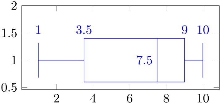
copy % Preamble: \pgfplotsset{width=7cm,compat=1.18}\usepgfplotslibrary{statistics} \begin{tikzpicture} \begin{axis}[y=1.5cm, ymax=2] \addplot+[boxplot] table[row sep=\\,y index=0] { data\\ 1\\ 2\\ 1\\ 5\\ 4\\ 10\\ 7\\ 10\\ 9\\ 8\\ 9\\ 9\\ } [above] node at (boxplot box cs: \boxplotvalue{lower whisker},1) {\pgfmathprintnumber{\boxplotvalue{lower whisker}}} node at (boxplot box cs: \boxplotvalue{lower quartile},1) {\pgfmathprintnumber{\boxplotvalue{lower quartile}}} node[left] at (boxplot box cs: \boxplotvalue{median},0.5) {\pgfmathprintnumber{\boxplotvalue{median}}} node at (boxplot box cs: \boxplotvalue{upper quartile},1) {\pgfmathprintnumber{\boxplotvalue{upper quartile}}} node at (boxplot box cs: \boxplotvalue{upper whisker},1) {\pgfmathprintnumber{\boxplotvalue{upper whisker}}} ; \end{axis} \end{tikzpicture}

Coordinate system boxplot whisker ¶

A coordinate system which is almost the same as boxplot box cs, except that it aligns at whisker extend instead of box extend.

The boxplot whisker cs accepts two arguments of the form boxplot whisker cs=(data coordinate, whisker-relative offset) where the first is a value of the box plot’s data (it is expressed in the same space as median or upper whisker).

The second argument is an offset expressed as signed multiple of whisker extend. An offset of \(0\) means to place the point exactly on the lower end of the whisker line. An offset of \(1\) places the point on the upper end of the whisker line. An offset of \(0.5\) places the point in the middle of the whisker line.



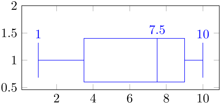
copy % Preamble: \pgfplotsset{width=7cm,compat=1.18}\usepgfplotslibrary{statistics} \begin{tikzpicture} \begin{axis}[y=1.5cm, ymax=2] \addplot+[boxplot] table[row sep=\\,y index=0] { data\\ 1\\ 2\\ 1\\ 5\\ 4\\ 10\\ 7\\ 10\\ 9\\ 8\\ 9\\ 9\\ } [above] node at (boxplot whisker cs:\boxplotvalue{lower whisker},1) {\pgfmathprintnumber{\boxplotvalue{lower whisker}}} node at (boxplot box cs: \boxplotvalue{median},1) {\pgfmathprintnumber{\boxplotvalue{median}}} node at (boxplot whisker cs:\boxplotvalue{upper whisker},1) {\pgfmathprintnumber{\boxplotvalue{upper whisker}}} ; \end{axis} \end{tikzpicture}

/pgfplots/boxplot/draw/lower whisker/.code={...} ¶

/pgfplots/boxplot/draw/upper whisker/.code={...} ¶

/pgfplots/boxplot/draw/whisker/.code={...} ¶

A couple of code keys which customize the stroke paths for whiskers.

The initial configuration is

copy \pgfplotsset{ boxplot/draw/lower whisker/.style={ /pgfplots/boxplot/draw/whisker= {\pgfplotsboxplotvalue{lower quartile}} {\pgfplotsboxplotvalue{lower whisker}} }, boxplot/draw/upper whisker/.style={ /pgfplots/boxplot/draw/whisker= {\pgfplotsboxplotvalue{upper quartile}} {\pgfplotsboxplotvalue{upper whisker}} }, boxplot/draw/whisker/.code 2 args={ \draw [/pgfplots/boxplot/every whisker/.try] (boxplot cs:#1) -- (boxplot cs:#2) (boxplot whisker cs:#2,0) -- (boxplot whisker cs:#2,1) ; }, }

The key draw/lower whisker key is used if and only if lower whisker has a numeric value. The key draw/upper whisker is used if and only if upper whisker has a value.

If one of lower quartile or upper quartile is empty, both are replaced by the following values:

lower quartile \(:=\) upper whisker and

upper quartile \(:=\) lower whisker.

Thus, if the box cannot be drawn but you only have whiskers, the two whiskers will be connected with each other.

/pgfplots/boxplot/draw/box/.code={...} ¶

A path which is used for every box.

copy \pgfplotsset{ boxplot/draw/box/.code={ \draw [/pgfplots/boxplot/every box/.try] (boxplot box cs:\pgfplotsboxplotvalue{lower quartile},0) rectangle (boxplot box cs:\pgfplotsboxplotvalue{upper quartile},1) ; }, }

It either lower quartile or upper quartile is empty, this key will not be invoked.

Note that draw/median will be invoked after this key.

/pgfplots/boxplot/draw/median/.code={...} ¶

A path which is used for every median. Its initial configuration is

copy \pgfplotsset{ boxplot/draw/median/.code={ \draw [/pgfplots/boxplot/every median/.try] (boxplot box cs:\pgfplotsboxplotvalue{median},0) -- (boxplot box cs:\pgfplotsboxplotvalue{median},1) ; }, }

This key will be omitted if median is empty.

/pgfplots/boxplot/draw/average/.code={...} ¶

The path which is used to visualize an average. The initial configuration is

copy \makeatletter \pgfplotsset{ boxplot/draw/average/.code={ \draw [/pgfplots/boxplot/every average/.try] \pgfextra % do NOT use \draw[mark=*] plot coordinates because % boxplots uses the same plot handler to draw its % outliers. \pgftransformshift{% % basic level access to 'boxplot box cs': \pgfplotsboxplotpointabbox {\pgfplotsboxplotvalue{average}} {0.5}% }% \pgfuseplotmark{\tikz@plot@mark}% \endpgfextra ; }, } \makeatother

This key will be omitted if average has an empty value (the default).

The key draw/average will be evaluated after draw/median and after draw/box.

/pgfplots/hist={options with hist/ prefix} ¶

\addplot+[hist={options with hist/ prefix}]

A histogram plot takes one-dimensional input data and counts the occurrence of values: it determines the data range \([\underline m,\overline m]\) and subdivides it into \(N\) equally sized bins with \((N+1)\) endpoints. Then, it counts the number of points falling into each bin. More precisely, it computes the \(N+1\) points \(\underline m =: x_0 < x_1 < \dotsb < x_N := \overline m\) using \(x_i := \underline m + i \cdot (\overline m - \underline m)/N\). Then, it creates the \(N+1\) coordinates \((x_i, y_i)\), \(i=0,\dotsc ,N-1\) by means of

\[ y_i := \begin {cases} \text {bincount}\bigl ([x_i,x_{i+1})\bigr )\Bigr ) & i < N \\ y_{N-1} & i = N, \end {cases} \]

i.e. the value of the last coordinate is replicated. This set of \((N+1)\) interval boundaries is then visualized by an ybar interval plot handler.



copy % Preamble: \pgfplotsset{width=7cm,compat=1.18}\usepgfplotslibrary{statistics} \begin{tikzpicture} \begin{axis}[ ybar interval, xticklabel= \pgfmathprintnumber\tick--\pgfmathprintnumber\nexttick ] \addplot+ [hist={bins=3}] table [row sep=\\,y index=0] { data\\ 1\\ 2\\ 1\\ 5\\ 4\\ 10\\ 7\\ 10\\ 9\\ 8\\ 9\\ 9\\ }; \end{axis} \end{tikzpicture}

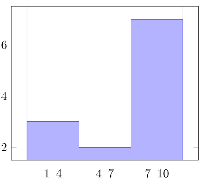
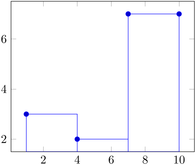
We see that hist={bins=3} takes a table with one column as input. The data values fall into the range \([1,10]\) which is partitioned into \(3\) intervals (of equal lengths). Finally, the number of points falling into each of the three bins is plotted. The xticklabel key shows the range (note that it works only in conjunction with x tick label as interval which has been enabled by ybar interval before). We see that there are \(3\) elements in the range \([1,4)\), \(2\) elements in the range \([4,7)\) and finally \(7\) elements in the range \([7,10]\).

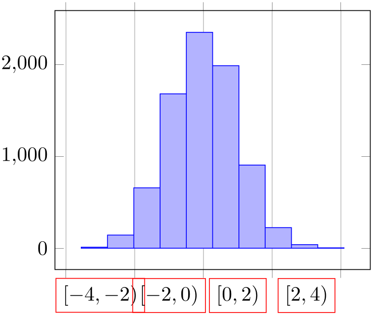
The bins are half-open intervals, i.e. the endpoint does not belong to the bin. Only the last bin contains its right end point.



copy % Preamble: \pgfplotsset{width=7cm,compat=1.18}\usepgfplotslibrary{statistics} \begin{tikzpicture} \begin{axis}[ ybar interval, xtick=,% reset from ybar interval xticklabel={ $[\pgfmathprintnumber\tick, \pgfmathprintnumber\nexttick)$ }], x tick label style={draw=red}, ] % a data file containing 8000 normally distributed % random numbers of mean 0 and variance 1 \addplot+ [hist={data=x}] file {plotdata/pgfplots.randn.dat}; \end{axis} \end{tikzpicture}

The hist plot type can be combined with plot expression as well: provide the usual expression as you would for a line plot. Then, configure the value for data=expression in dependence of x, y, or z:



copy % Preamble: \pgfplotsset{width=7cm,compat=1.18}\usepgfplotslibrary{statistics} \begin{tikzpicture} \begin{axis}[ tiny, height=4cm,width=12cm, ybar interval, ymin=0, xmin=0,xmax=1, axis on top, extra x ticks={0,1}, extra x tick style={ grid=none, x tick label as interval=false, xticklabel={$\pgfmathprintnumber\tick$} }, xticklabel={$[\pgfmathprintnumber[fixed]\tick,\cdot)$}, ] \addplot+ [samples=200,hist] {rnd}; \end{axis} \end{tikzpicture}

The example uses the rnd method of pgf which defines y to contain uniform random numbers in the range \([0,1]\). Then, it configures hist. Note that hist has the default data=y such that it uses the y coordinate as input. Note furthermore that the x value is effectively ignored here. The options after \begin{axis}[...] are mainly to scale the graphics and to insert the right limits. The extra x ticks method is inserted to demonstrate how to add further tick marks without affecting the overall layout. Note that the extra x tick style sets x tick label as interval=false to disable the special tick handling which is active for the rest of the plot.

The following keys configure hist. If they are provided inside of options, the common key prefix hist/ can be omitted.

/pgfplots/hist/data={expression} (initially y) ¶

Tells hist how to get its data. The common idea is to provide a mathematical expression which depends on data supplied by the \addplot statement. For example, if you have \addplot expression, the expression may depend upon x, y or z. In case of an \addplot table input routine, the expression can employ \thisrow{colname} to access the currently active table row in the designated column.

It is also possible to avoid invocations of the math parser. Use hist/data value={value} instead to do so. Here, value should be of a numeric constant.

The initial configuration employs what would usually become the final y coordinate as input (to be more precise, the initial value is data value=\pgfkeysvalueof{/data point/y}).

/pgfplots/hist/data min={min value} (initially /pgfplots/xmin) ¶

/pgfplots/hist/data max={max value} (initially /pgfplots/xmax) ¶

Allows to provide the min/max values (the \(\underline m\) and \(\overline m\)) values manually.

If empty, these values will be deduced from the input data range.

The resulting interval will be split into hist/bins intervals.

The initial configuration uses any provided data limits, i.e. the (natural) choices hist/data min=xmin and hist/data max=xmax.

/pgfplots/hist/bins={number of intervals} (initially 10) ¶

Specifies the number of intervals to use.

/pgfplots/hist/intervals={true,false} (initially true) ¶

If intervals=true (the initial configuration), hist will generate \(N+1\) coordinates, with

\[ \underline m = x_0 < x_1 < \dotsb < x_{N} = \overline m \]

where \([\underline m,\overline m]\) is the data range. In this case, the data points for \(x_{N-1}\) and \(x_N\) will get the same value, namely the number of elements in the last bin. This is (only) useful in conjunction with const plot or ybar interval.

If intervals=false, the last data point will be omitted and exactly \(N\) coordinates will be generated. In this case, the right end point is not returned explicitly.

/pgfplots/hist/cumulative={true,false} (initially false) ¶

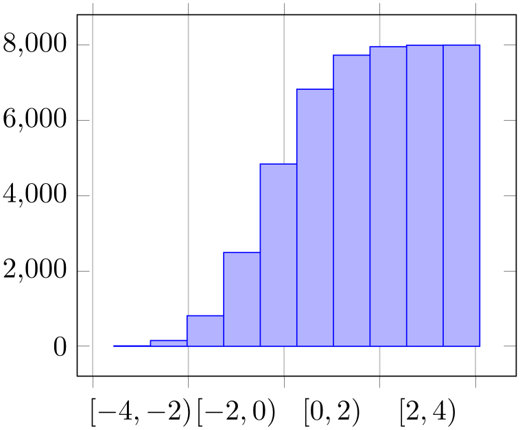
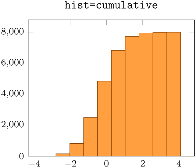
Allows to compute a cumulative histogram.

A cumulative histogram uses the sum of all previous bins and the current one as final value.

Here is the example from above, this time with hist/cumulative:



copy % Preamble: \pgfplotsset{width=7cm,compat=1.18}\usepgfplotslibrary{statistics} \begin{tikzpicture} \begin{axis}[ ybar interval, xtick=,% reset from ybar interval xticklabel={ $[\pgfmathprintnumber\tick, \pgfmathprintnumber\nexttick)$ }], ] % a data file containing 8000 normally distributed % random numbers of mean 0 and variance 1 \addplot+ [hist={data=x,cumulative}] file {plotdata/pgfplots.randn.dat}; \end{axis} \end{tikzpicture}

/pgfplots/hist/density={true,false} (initially false) ¶

An extension by Jürnjakob Dugge

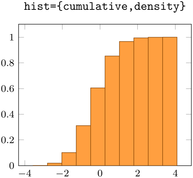
Enables density estimation mode. If hist/density is active, the resulting data points will be renormalized such that the overall “mass” equals \(1\).



copy % Preamble: \pgfplotsset{width=7cm,compat=1.18}\usepgfplotslibrary{statistics} \begin{tikzpicture} \begin{axis}[small,ymin=0,title=\texttt{hist}] \addplot [ hist, fill=orange!75, draw=orange!50!black] table [y index=0] {plotdata/pgfplots.randn.dat}; \end{axis} \end{tikzpicture} % \begin{tikzpicture} \begin{axis}[small,ymin=0, title=\texttt{hist=density}] \addplot [ hist=density, fill=orange!75, draw=orange!50!black] table [y index=0] {plotdata/pgfplots.randn.dat}; \end{axis} \end{tikzpicture}

The keys hist/density and hist/cumulative can be combined as well:



copy % Preamble: \pgfplotsset{width=7cm,compat=1.18}\usepgfplotslibrary{statistics} \begin{tikzpicture} \begin{axis}[small,ymin=0, title=\texttt{hist=cumulative}] \addplot [ hist=cumulative, fill=orange!75, draw=orange!50!black] table [y index=0] {plotdata/pgfplots.randn.dat}; \end{axis} \end{tikzpicture} % \begin{tikzpicture} \begin{axis}[small,ymin=0, title=\texttt{hist=\{cumulative,density\}}] \addplot [ hist={cumulative,density}, fill=orange!75, draw=orange!50!black] table [y index=0] {plotdata/pgfplots.randn.dat}; \end{axis} \end{tikzpicture}

/pgfplots/hist/handler(style, initially ybar interval) ¶

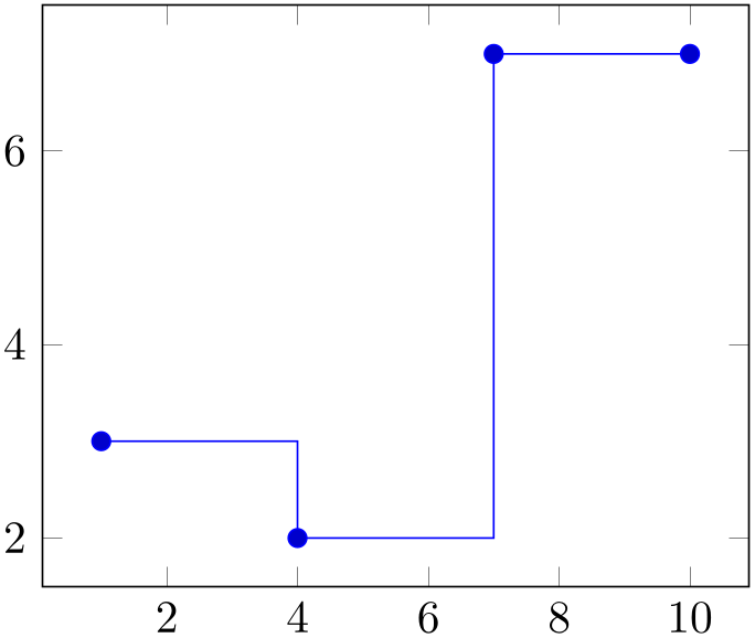
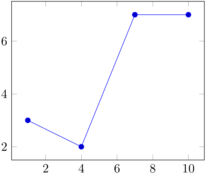
Allows to change the way the generated coordinates are visualized. The hist/handler key is a style, so use hist/handler/.style={const plot} to change it.



copy % Preamble: \pgfplotsset{width=7cm,compat=1.18}\usepgfplotslibrary{statistics} \begin{tikzpicture} \begin{axis} \addplot+ [ hist={bins=3}, ] table [row sep=\\,y index=0] { data\\ 1\\ 2\\ 1\\ 5\\ 4\\ 10\\ 7\\ 10\\ 9\\ 8\\ 9\\ 9\\ }; \end{axis} \end{tikzpicture}



copy % Preamble: \pgfplotsset{width=7cm,compat=1.18}\usepgfplotslibrary{statistics} \begin{tikzpicture} \begin{axis} \addplot+ [ hist={ bins=3, handler/.style={const plot}, }, ] table [row sep=\\,y index=0] { data\\ 1\\ 2\\ 1\\ 5\\ 4\\ 10\\ 7\\ 10\\ 9\\ 8\\ 9\\ 9\\ }; \end{axis} \end{tikzpicture}



copy % Preamble: \pgfplotsset{width=7cm,compat=1.18}\usepgfplotslibrary{statistics} \begin{tikzpicture} \begin{axis} \addplot+ [ hist={ bins=3, handler/.style={sharp plot}, }, ] table [row sep=\\,y index=0] { data\\ 1\\ 2\\ 1\\ 5\\ 4\\ 10\\ 7\\ 10\\ 9\\ 8\\ 9\\ 9\\ }; \end{axis} \end{tikzpicture}

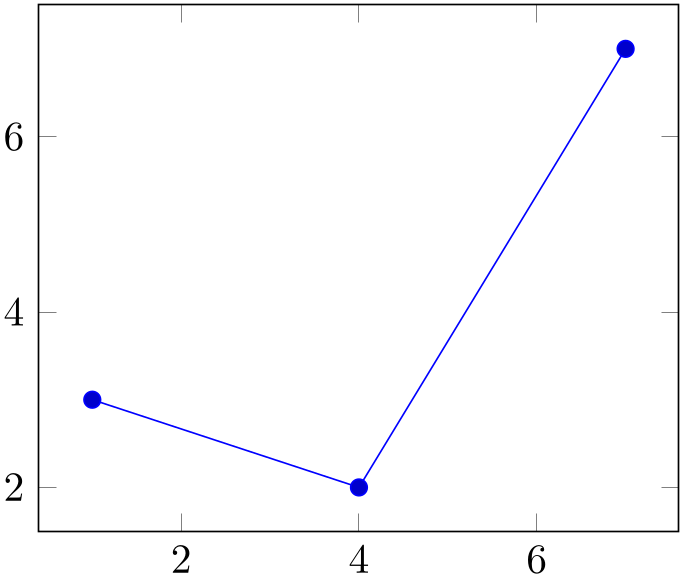
Note that sharp plot might benefit from intervals=false:



copy % Preamble: \pgfplotsset{width=7cm,compat=1.18}\usepgfplotslibrary{statistics} \begin{tikzpicture} \begin{axis} \addplot+ [ hist={ bins=3, handler/.style={sharp plot}, intervals=false, }, ] table [row sep=\\,y index=0] { data\\ 1\\ 2\\ 1\\ 5\\ 4\\ 10\\ 7\\ 10\\ 9\\ 8\\ 9\\ 9\\ }; \end{axis} \end{tikzpicture}

/pgfplots/hist/data filter/.code={...} ¶

Allows to define coordinate filters, similar to the coordinate filter key x filter described in Section 4.22. The argument #1 is the coordinate as it has been found after processing hist/data. The code is supposed to assign \pgfmathresult to contain the result. If \pgfmathresult is empty afterwards, it will be skipped. Otherwise, it is supposed to contain a number.

This filter is applied before the histogram is computed. Note that x filter and y filter are applied after the histogram is computed.

Note that predefined styles like each nth point can also be applied to hist/data if

• 1. an asterisk ‘*’ is appended to the predefined style’s name and

• 2. the first argument to the style is hist/data.

For example, each nth point*={hist/data}{2} will skip each second input value of hist/data (try it out).

/pgfplots/hist/data coord trafo/.code={...} ¶

/pgfplots/hist/data coord inv trafo/.code={...} ¶

These keys work in the same way as for x coord trafo and x coord inv trafo. They are applied to the hist/data value before the histogram is evaluated and after the result value is assigned, respectively.

Note that hist will apply the hist/data coord inv trafo before it visualizes its results. Consequently, it may be necessary to assign a similar transformation to x coord trafo as well.

See the documentation of x coord trafo for more information about custom transformations.

/pgfplots/hist/symbolic coords={list} ¶

A style which enables symbolic x coords for an axis containing hist plots:



copy % Preamble: \pgfplotsset{width=7cm,compat=1.18}\usepgfplotslibrary{statistics} \begin{tikzpicture} \begin{axis}[ ybar interval, hist/symbolic coords={A,B,C,D,E,F,G,H,I,J}, xticklabel={[\tick--\nexttick[}], ] \addplot+ [ hist={bins=3}, ] table [row sep=\\,y index=0] { data\\ A\\ B\\ A\\ D\\ F\\ J\\ G\\ J\\ I\\ H\\ I\\ I\\ }; \end{axis} \end{tikzpicture}

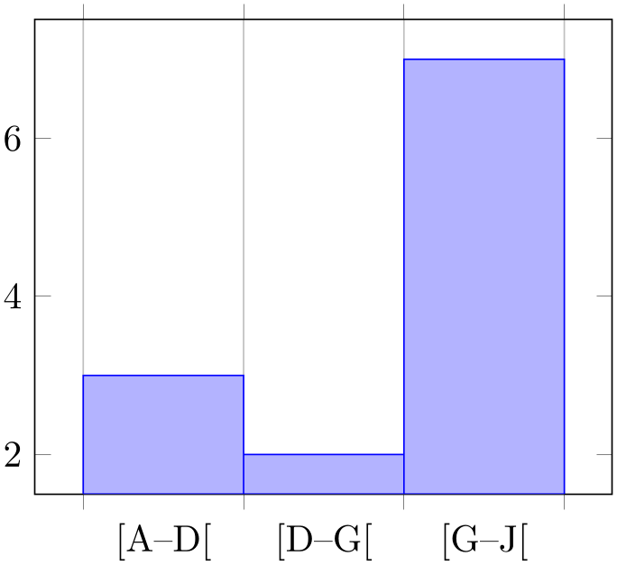
The style does two things: first, it defines hist/data coord trafo and hist/data coord inv trafo, then, it calls symbolic x coords with the same argument.

Attention:

do not use hist/data=x or other symbolic values as input when you have symbolic coords. Rather than symbolic values, you need to provide expandable values like \pgfkeysvalueof{/data point/x} (which has the same effect, but directly expands to the correct value).

Please refer to the documentation of symbolic x coords for further details about symbolic coordinates.