Manual for Package pgfplots
2D/3D Plots in LATeX, Version 1.18.2
https://github.com/pgf-tikz/pgfplots
Related Libraries
5.13Ternary Diagrams
-
\usepgfplotslibrary{ternary} % LaTeX and plain TeX 
-
\usepgfplotslibrary[ternary] % ConTeXt 
-
\usetikzlibrary{pgfplots.ternary} % LaTeX and plain TeX 
-
\usetikzlibrary[pgfplots.ternary] % ConTeXt 
A library to draw ternary diagrams.
A ternary diagram visualizes three-component systems such that the sum of them yields \(100\%\). Ternary diagrams are triangular axes.
5.13.1Ternary Axis
-
\begin{ternaryaxis}[
 options
 ]
]
-
 environment contents
-
\end{ternaryaxis} 
The axis environment for ternary axes.
% Preamble: \pgfplotsset{width=7cm,compat=1.18}\usepgfplotslibrary{ternary}
\begin{tikzpicture}
\begin{ternaryaxis}
                        \addplot3
                    coordinates {
(0.81, 0.19, 0.00)
(0.76, 0.17, 0.07)
(0.66, 0.16, 0.16)
(0.76, 0.07, 0.17)
(0.81, 0.00, 0.19)
};
                        \addplot3
                    coordinates {
(0.85, 0.15, 0.00)
(0.82, 0.13, 0.05)
(0.73, 0.14, 0.13)
(0.82, 0.06, 0.13)
(0.84, 0.00, 0.16)
};
\legend{$10$\textdegree, $20$\textdegree}
\end{ternaryaxis}
\end{tikzpicture}
A ternaryaxis works with relative coordinates: each data point consists of three components \(x\), \(y\), \(z\). Their sum forms a compound entity which has \(100\%\) (of whatever). In the standard configuration, we have \(x,y,z \in [0,1]\). The unit interval is not necessary: you can as well choose absolute data ranges \(x \in [x_{\min },x_{\max }]\), \(y \in [y_{\min },y_{\max }]\) and \(z \in [z_{\min },z_{\max }]\). The important thing is that the relative values \(\tilde x := \frac {x-x_{\min }}{x_{\max } - x_{\min }}\), \(\tilde y := \frac {y-y_{\min }}{y_{\max } - y_{\min }}\), \(\tilde z := \frac {z-z_{\min }}{z_{\max } - z_{\min }}\) sum up to \(100\%\), i.e. \(\tilde x + \tilde y + \tilde z = 1\). Thus, pgfplots computes \(\tilde x\), \(\tilde y\) and \(\tilde z\) and interprets them as barycentric (triangular) coordinates.
For this to work, it is crucial to provide xmin, xmax, ymin, ymax and zmin, zmax precisely! The initial configuration fixes them to the unit interval.
What happens behind the scenes is that a data point \((x,y,z)\) is placed at \(X,Y\) determined by
\(\seteqnumber{0}{}{0}\)\begin{align*} \begin{bmatrix} X(x,y,z)\\ Y(x,y,z) \end {bmatrix} &= \tilde x A + \tilde y B + \tilde z C \\ &= \begin{bmatrix} \frac 12 {\tilde x+2 \tilde z}\\ \frac {\sqrt 3}{2} {\tilde x} \end {bmatrix} \end{align*} where \(A=(\nicefrac 12,\nicefrac {\sqrt 3}{2})\) is top corner of the triangle, \(B=(0,0)\) the lower left and \(C=(1,0)\) the lower right one. The \(\tilde y\) component is not really necessary due to the linear dependency \(\tilde x+\tilde y+\tilde z=1\).
The input coordinate \((100\%,0\%,0\%)\) is mapped to \(A\), the input coordinate \((0\%,100\%,0\%)\) to \(B\) and \((0\%,0\%,100\%)\) to \(C\) (Acrobat Reader: click into the axis to verify it).

% Preamble: \pgfplotsset{width=7cm,compat=1.18}\usepgfplotslibrary{ternary}
\begin{tikzpicture}
\begin{ternaryaxis}[xlabel=A,ylabel=B,zlabel=C]
                        \addplot3
                    coordinates {
(0.81, 0.19, 0.00)
(0.76, 0.17, 0.07)
(0.66, 0.16, 0.16)
(0.76, 0.07, 0.17)
(0.81, 0.00, 0.19)
};
                        \addplot3
                    coordinates {
(0.85, 0.15, 0.00)
(0.82, 0.13, 0.05)
(0.73, 0.14, 0.13)
(0.82, 0.06, 0.13)
(0.84, 0.00, 0.16)
};
\node [pin=130:Deduced $z$,draw=black] at (0.2,0.2) {};
\legend{$10$\textdegree, $20$\textdegree}
\end{ternaryaxis}
\end{tikzpicture}
A ternaryaxis can contain zero, one or more \addplot3 commands, just as a usual axis. In case you provide only two-dimensional coordinates (for example using \addplot or axis cs), the third component is deduced automatically such that components sum to \(100\%\). The \addplot3 command can use any of the accepted input formats, for example using coordinates, table, expression or whatever – but the input is always interpreted as barycentric coordinates (three components summing up to \(100\%\)).

% Preamble: \pgfplotsset{width=7cm,compat=1.18}\usepgfplotslibrary{ternary}
\begin{tikzpicture}
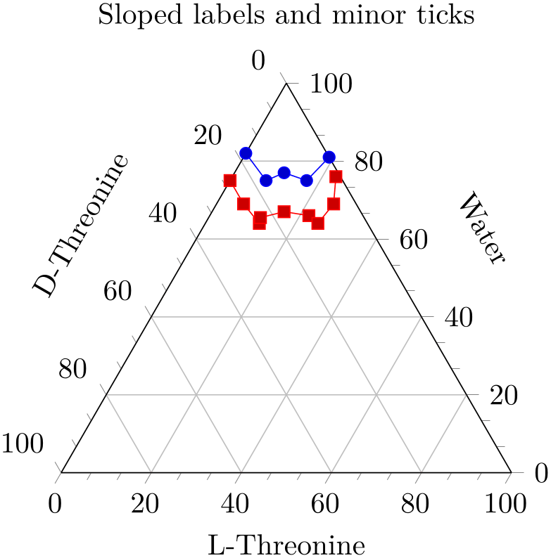
\begin{ternaryaxis}[
                    title=Sloped labels and minor
                ticks,
xlabel=Water,
ylabel=D-Threonine,
zlabel=L-Threonine,
label style={sloped},
minor tick num=2,
]
                    \addplot3
                coordinates {
(0.82, 0.18, 0.00)
(0.75, 0.17, 0.08)
(0.77, 0.12, 0.11)
(0.75, 0.08, 0.17)
(0.81, 0.00, 0.19)
};
                    \addplot3
                coordinates {
(0.75, 0.25, 0.00)
(0.69, 0.25, 0.06)
(0.64, 0.24, 0.12)
(0.655, 0.23, 0.115)
(0.67, 0.17, 0.16)
(0.66, 0.12, 0.22)
(0.64, 0.11, 0.25)
(0.69, 0.05, 0.26)
(0.76, 0.01, 0.23)
};
\end{ternaryaxis}
\end{tikzpicture}
% Preamble: \pgfplotsset{width=7cm,compat=1.18}\usepgfplotslibrary{ternary}
\begin{tikzpicture}
\begin{ternaryaxis}[
                    title=Sloped labels and minor
                grids,
xlabel=Water,
ylabel=D-Threonine,
zlabel=L-Threonine,
label style={sloped},
minor tick num=2,
grid=both,
]
                    \addplot3
                coordinates {
(0.82, 0.18, 0.00)
(0.75, 0.17, 0.08)
(0.77, 0.12, 0.11)
(0.75, 0.08, 0.17)
(0.81, 0.00, 0.19)
};
                    \addplot3
                coordinates {
(0.75, 0.25, 0.00)
(0.69, 0.25, 0.06)
(0.64, 0.24, 0.12)
(0.655, 0.23, 0.115)
(0.67, 0.17, 0.16)
(0.66, 0.12, 0.22)
(0.64, 0.11, 0.25)
(0.69, 0.05, 0.26)
(0.76, 0.01, 0.23)
};
\end{ternaryaxis}
\end{tikzpicture}
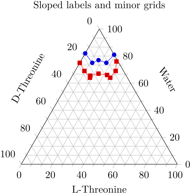
A ternaryaxis supports (most of) the
pgfplots axis interface, among them the
grid option, the
xtick={ positions
 } way to provide ticks, including extra x ticks and
its variants. Of course, it can also contain any of the mark, color and
cycle list options of a normal axis.
The following example is a (crude) copy of an example of
ternary2.html (sv.vt.edu)
and uses area style to change cycle list and the legend appearance.
% Preamble: \pgfplotsset{width=7cm,compat=1.18}\usepgfplotslibrary{ternary}
\begin{tikzpicture}
\begin{ternaryaxis}[
title=Want--be--Stainless Steel,
xlabel=Weight Percent Chromium,
ylabel=Weight Percent Iron,
zlabel=Weight Percent Nickel,
label style=sloped,
area style,
]
                    \addplot3
                table {
A B C
1 0 0
0.5 0.4 0.1
0.45 0.52 0.03
0.36 0.6 0.04
0.1 0.9 0
};
\addlegendentry{Cr}
                    \addplot3
                table {
A B C
1 0 0
0.5 0.4 0.1
0.28 0.35 0.37
0.4 0 0.6
};
\addlegendentry{Cr+$\gamma$FeNi}
                    \addplot3
                table {
0.4 0 0.6
0.28 0.35 0.37
0.25 0.6 0.15
0.1 0.9 0
0 1 0
0 0 1
};
\addlegendentry{$\gamma$FeNi}
                    \addplot3
                table {
0.1 0.9 0
0.36 0.6 0.04
0.25 0.6 0.15
};
\addlegendentry{Cr+$\gamma$FeNi}
                    \addplot3
                table {
0.5 0.4 0.1
0.45 0.52 0.03
0.36 0.6 0.04
0.25 0.6 0.15
0.28 0.35 0.37
};
\addlegendentry{$\sigma$+$\gamma$FeNi}
\node [inner sep=0.5pt,circle,draw,fill=white,pin=-15:\footnotesize Stainless Steel]
at (0.18,0.74,0.08) {};
\end{ternaryaxis}
\end{tikzpicture}
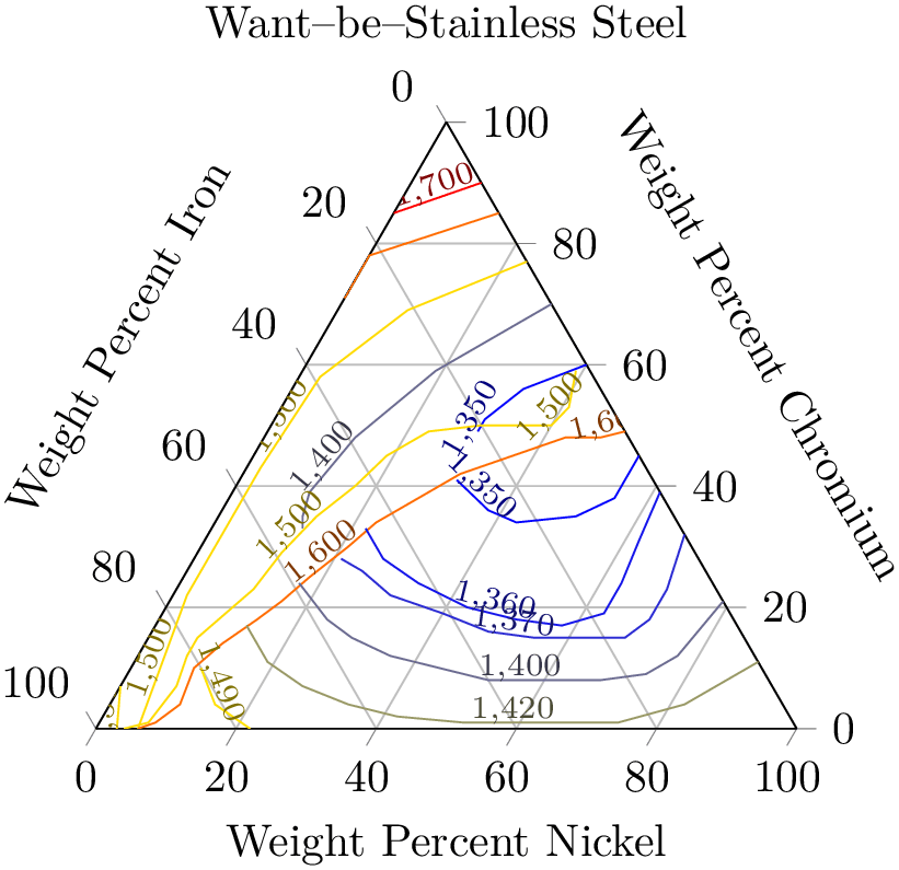
Ternary plots can also use contour prepared to plot contour lines. The following example is a (crude) copy of an example of
ternary2.html (sv.vt.edu):
% Preamble: \pgfplotsset{width=7cm,compat=1.18}\usepgfplotslibrary{ternary}
\begin{tikzpicture}
\begin{ternaryaxis}[
title=Want--be--Stainless Steel,
xlabel=Weight Percent Chromium,
ylabel=Weight Percent Iron,
zlabel=Weight Percent Nickel,
label style=sloped,
]
% plotdata/pgfplotsternary.example1.dat:
%
% Chromium Iron Nickel Temperature
% 0.90 0.0 0.10 1700
% 0.85 0.14 0.00 1700
%
% 0.85 0.00 0.15 1600
% 0.78 0.22 0.00 1600
% 0.71 0.29 0.00 1600
% ...
\addplot3 [contour prepared={labels over line},
point meta=\thisrow{Temperature}]
                            table
                [x=Chromium,y=Iron,z=Nickel]
{plotdata/pgfplotsternary.example1.dat};
\end{ternaryaxis}
\end{tikzpicture}
The contour prepared={labels over line} installs the display style contour/labels over line and expects precomputed contour lines from the input stream. Here, the input stream is a table, consisting of the three relative components for Chromium, Iron and Nickel – and the point meta is set to be the Temperature column. The contour prepared style uses the \((x,y,z)\) coordinate to plot the data point and the point meta to determine contour labels (the initial configuration of contour prepared is to use point meta=z). The output thus allows to use both barycentric coordinates (ternary components) and contour labels.
-
/pgfplots/ternary limits relative=true|false (initially true) 
-
/pgfplots/ternary relative limits=true|false (initially true) 
Allows to switch tick labels between relative numbers in the range \([0,100]\) or absolute numbers.
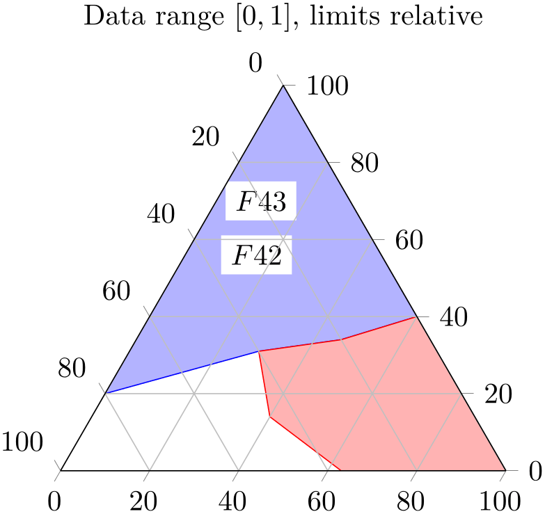
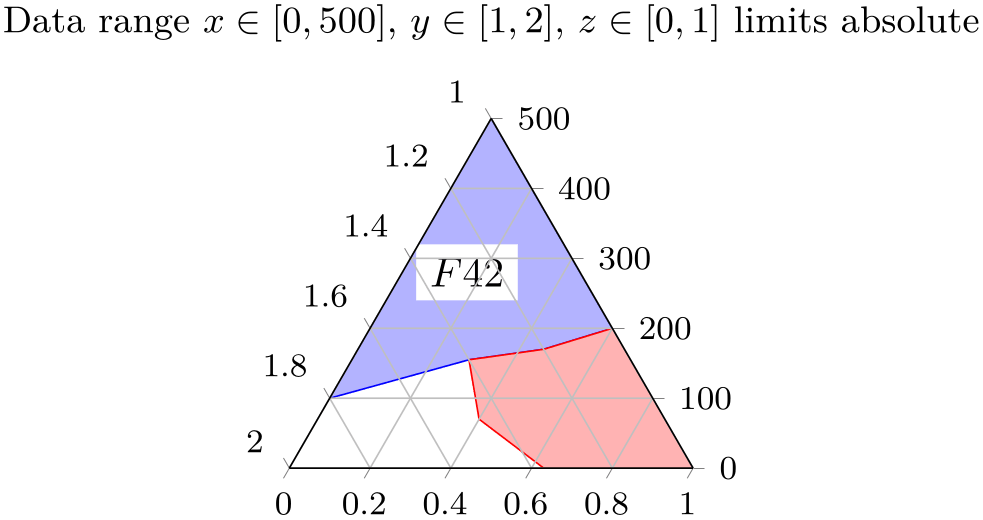
The choice ternary limits relative=true accepts data in any input number range, for example \((x,y,z) \in [0,1]^3\), or \((x,y,z) \in [0,100]^3\) or in any absolute scala of the form \(x_i \in [\underline x_i,\overline x_i]\) for \(x_i \in \{x,y,z\}\) (remember that it is crucial to communicate these limits to pgfplots explicitly using xmin, xmax, ymin, ymax and zmin, zmax such that relative coordinates can be computed, see the description above for details). In every case, relative tick labels are drawn, i.e. tick labels in the range \([0,100]\).

% Preamble: \pgfplotsset{width=7cm,compat=1.18}\usepgfplotslibrary{ternary}
\begin{tikzpicture}
\begin{ternaryaxis}[
ternary limits relative,
                        title={Data range
                    $[0,1]$, limits relative},
area style,
]
                        \addplot3
                    coordinates {
(0.2,0.8,0)
(0.31,0.4,0.29)
(0.34,0.2,0.46)
(0.4,0,0.6)
(1,0,0)
};
                        \addplot3
                    coordinates {
(0.4,0,0.6)
(0.34,0.2,0.46)
(0.31,0.4,0.29)
(0.14,0.46,0.4)
(0,0.37,0.63)
(0,0,1)
};
\node [fill=white]
at (axis cs:0.56,0.28,0.16) {$F 42$};
\node [fill=white]
at (0.7,0.2) {$F 43$};
\end{ternaryaxis}
\end{tikzpicture}

% Preamble: \pgfplotsset{width=7cm,compat=1.18}\usepgfplotslibrary{ternary}
\begin{tikzpicture}
\begin{ternaryaxis}[
xmax=500,ymin=1,ymax=2,
ternary limits relative,
                        title={Data range
                    $x\in[0,500]$,
$y\in[1,2]$, $z\in[0,1]$ limits relative},
area style,
]
                        \addplot3
                    coordinates {
(100,1.8,0)
(155,1.4,0.29)
(170,1.2,0.46)
(200,1,0.6)
(500,1,0)
};
                        \addplot3
                    coordinates {
(200,1,0.6)
(170,1.2,0.46)
(155,1.4,0.29)
(70,1.46,0.4)
(0,1.37,0.63)
(0,1,1)
};
\node [fill=white]
at (axis cs:280,1.28,0.16) {$F 42$};
\node [fill=white]
at (0.7,0.2) {$F 43$};
\end{ternaryaxis}
\end{tikzpicture}
The choice ternary limits relative=false accepts the same data ranges, but it draws tick labels in the very same data ranges.
% Preamble: \pgfplotsset{width=7cm,compat=1.18}\usepgfplotslibrary{ternary}
\begin{tikzpicture}
\begin{ternaryaxis}[
ternary limits relative=false,
xmax=500,ymin=1,ymax=2,
                        title={Data range
                    $x\in[0,500]$,
$y\in[1,2]$, $z\in[0,1]$ limits absolute},
                        footnotesize, % just for
                    the sake of demonstration...
area style,
]
                        \addplot3
                    coordinates {
(100,1.8,0)
(155,1.4,0.29)
(170,1.2,0.46)
(200,1,0.6)
(500,1,0)
};
                        \addplot3
                    coordinates {
(200,1,0.6)
(170,1.2,0.46)
(155,1.4,0.29)
(70,1.46,0.4)
(0,1.37,0.63)
(0,1,1)
};
\node [fill=white]
at (axis cs:280,1.28,0.16) {$F 42$};
\node [fill=white]
at (0.7,0.2) {$F 43$};
\end{ternaryaxis}
\end{tikzpicture}
-
Coordinate system cartesian cs 
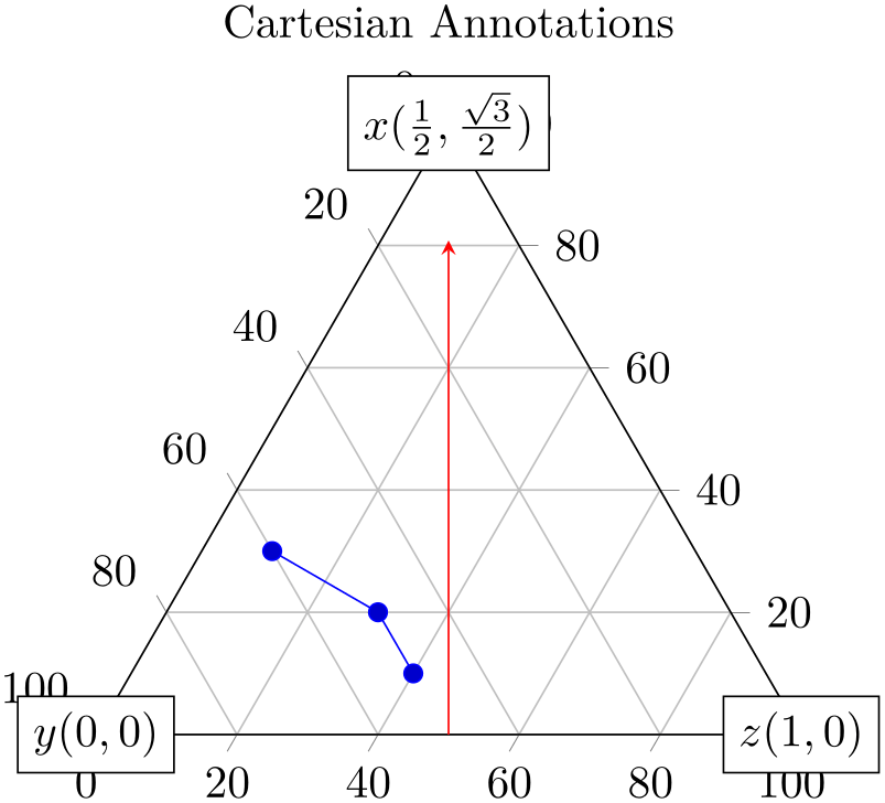
A coordinate system which allows Cartesian coordinates. The lower left point has coordinate \((0,0)\), the lower right point has \((1,0)\) and the upper point of the triangle is at \((\nicefrac {1}{2}, \nicefrac {\sqrt 3}{2})\).
% Preamble: \pgfplotsset{width=7cm,compat=1.18}\usepgfplotslibrary{ternary}
\begin{tikzpicture}
\begin{ternaryaxis}[
title=Cartesian Annotations,
clip=false,
]
                        \addplot3
                    coordinates {
(0.1,0.5,0.4)
(0.2,0.5,0.3)
(0.3,0.6,0.1)
};
\node [fill=white,draw]
at (cartesian cs:0,0) {$y (0,0)$};
\node [fill=white,draw]
at (cartesian cs:1,0) {$z (1,0)$};
\node [fill=white,draw]
at (cartesian cs:0.5,{sqrt(3)/2})
{$x (\frac12,\frac{\sqrt3}{2})$};
\draw [red,-stealth]
(cartesian cs:0.5,0)
-- (cartesian cs:0.5,0.7);
\end{ternaryaxis}
\end{tikzpicture}
Note that you need to prefix the coordinate with cartesian cs:; otherwise pgfplots will interpret the coordinate as ternary (since compat=1.11).
-
/pgfplots/every ternary axis(style, no value) 
A style which is installed at the beginning of every ternary axis. It is used to adjust some of the pgfplots keys to fit the triangular shape.
The initial configuration is
\pgfplotsset{
every ternary axis/.style={
tick align=outside,
grid=major,
xticklabel style={anchor=west},
every 3d description/.style={},
every axis x label/.style={at={(ticklabel cs:0.5)},anchor=near ticklabel},
every axis y label/.style={at={(ticklabel cs:0.5)},anchor=near ticklabel},
every axis z label/.style={at={(ticklabel cs:0.5)},anchor=near ticklabel},
every x tick scale label/.style=
{at={(xticklabel cs:0.95,5pt)},anchor=near xticklabel,inner sep=0pt},
every y tick scale label/.style=
{at={(yticklabel cs:0.95,5pt)},anchor=near yticklabel,inner sep=0pt},
every z tick scale label/.style=
{at={(yticklabel cs:0.95,5pt)},anchor=near yticklabel,inner sep=0pt},
every axis title shift=15pt,
every axis legend/.style={
cells={anchor=center},
                                inner xsep=3pt,inner
                    ysep=2pt,nodes={inner sep=2pt,text depth=0.15em},
shape=rectangle,
fill=white,
draw=black,
at={(1.03,1.03)},
anchor=north west,
},
annot/point format 3d/.initial={(\% .2f, \%.2f, \%.2f)},
},
}
5.13.2Tieline Plots
-
/tikz/tieline={
 options with tieline/ prefix
 }
}
-
\addplot+[tieline={
 options with tieline/ prefix
 }]
}]
-
/pgfplots/table/tie end x={
 colname
 } (initially empty)
-
/pgfplots/table/tie end y={
 colname
 } (initially empty)
-
/pgfplots/table/tie end z={
 colname
 } (initially empty)
-
/pgfplots/table/tie end x index={
 col index
 } (initially empty)
-
/pgfplots/table/tie end y index={
 col index
 } (initially empty)
-
/pgfplots/table/tie end z index={
 col index
 } (initially empty)
-
/pgfplots/tieline/each nth tie={
 number
 } (initially empty)
-
/pgfplots/tieline/tieline style={
 options
 }
}
-
/pgfplots/tieline/curve style={
 options
 }
}
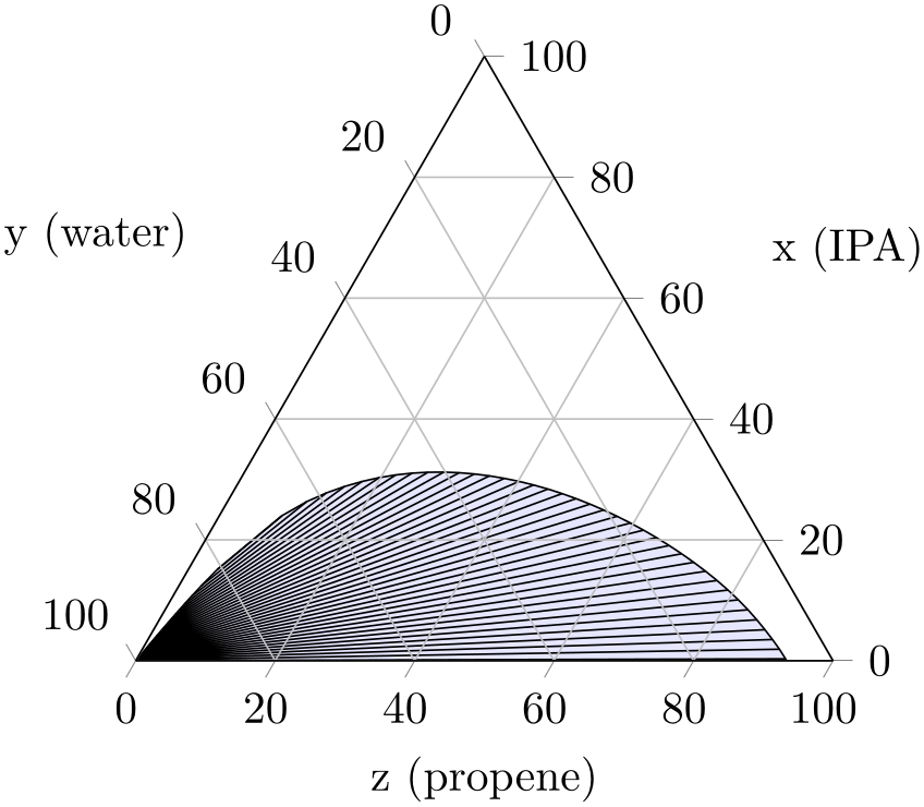
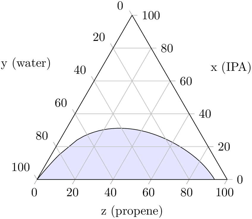
A plot handler for use in ternary diagrams which plots tie lines and binodal curves.
On input, it accepts pairs of coordinates, \(A^{(i)}=(A_x^{(i)},A_y^{(i)},A_z^{(i)})\) and \(B^{(i)}=(B_x^{(1)},B_y^{(2)},B_z^{(3)})\), for \(i=1,\dotsc ,N\) (i.e. it requires a total of six coordinates, perhaps plus additional color data).
On output, it connects the pairs, i.e. for every fixed \(i=1,\dotsc ,N\), it connects \(A^{(i)}\) – \(B^{(i)}\) (the so-called “tie lines”). In addition, it also draws the binodal curve, which is made up by connecting all \(A^{(i)}\) and then, in reverse ordering, all \(B^{(i)}\): \(A^{(1)}\) – \(A^{(2)}\) – \(\dotsb \) – \(A^{(N)}\) – \(B^{(N)}\) – \(B^{(N-1)}\) – \(\dotsb \) – \(B^{(1)}\):
% Preamble: \pgfplotsset{width=7cm,compat=1.18}\usepgfplotslibrary{ternary}
\begin{tikzpicture}
\begin{ternaryaxis}[
                        xlabel=x
                    (IPA),
                        ylabel=y
                    (water),
zlabel=z (propene),
axis on top,
]
% plotdata/ternary_data.txt is a table of the form
% A_propene A_water A_IPA B_propene B_water B_IPA
% 0.0009 0.9990 0 0.9333 0.0667 0
% 0.0009 0.9988 0.0002 0.9303 0.0665 0.0032
% 0.0011 0.9975 0.0013 0.9135 0.0673 0.0191
% 0.0013 0.9962 0.0024 0.8956 0.0693 0.0351
% ...
\addplot3 [tieline,fill=blue!10]
table [x=A_IPA,y=A_water,z=A_propene]
{plotdata/ternary_data.txt};
\end{ternaryaxis}
\end{tikzpicture}
We see that each input line has six columns, and each six columns are taken into account (this is different from other plot handlers!). The six columns make up the three components of the \(A\) and \(B\) points, respectively. In the example above, we used explicit column names and provided \(A_x\) using x=A_IPA, \(A_y\) using y=A_water and \(A_z\) using z=A_propene. Note that these keys are the common input method for \addplot table; they are nothing special (that means we could also use x index instead). The three columns for \(B\) can be provided manually (see below), or deduced automatically: in our case, the value for \(B_x\) has been found in the third column after x=A_IPA (which is B_IPA); the value for \(B_y\) has been found in the third column after y=A_water and \(B_z\) is made up from the third column after z=A_propene. In other words, the \(B\) value is searched (by default) by adding \(3\) to the column index of the respective \(A\) coordinate.
You do not need to provide any column names; in this case, the first three columns make up \(A\) (in the order of appearance) and the following three make up \(B\).
The only supported input type for tieline plots is table input. It is optimized to use \addplot3 table (as described above). To use the two-dimensional variant \addplot table, you need to tell pgfplots explicitly which columns make up \(A_x,A_y,B_x,B_y\); the \(z\)-coordinates are deduced automatically such that the result sums to \(100\%\).
These keys can be used to provide column names or column indices for \(B_x\), \(B_y\) and \(B_z\), respectively. They can be provided like
\addplot3[tieline] table[tie end y=B_water] ....
Note that the tie end x keys are only available if the tieline option has been used before.
The values for \(A\) are provided with table/x, table/x index and its variants as for any other plot type.
The tieline plot handler accepts several options to customize the
appearance. You can provide them as argument after tieline, using tieline={ options
 }. In this case, the tieline/ prefix can be omitted. The keys are described in the following:
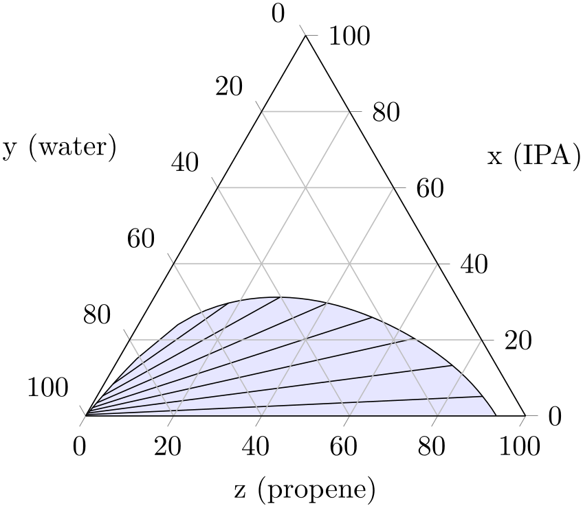
Allows to draw only each \(n\)th tie line, even though the binodal curve uses all provided coordinates:
% Preamble: \pgfplotsset{width=7cm,compat=1.18}\usepgfplotslibrary{ternary}
\begin{tikzpicture}
\begin{ternaryaxis}[
                            xlabel=x
                        (IPA),
                            ylabel=y
                        (water),
zlabel=z (propene),
axis on top,
]
% plotdata/ternary_data.txt is a table of the form
% A_propene A_water A_IPA B_propene B_water B_IPA
% 0.0009 0.9990 0 0.9333 0.0667 0
% 0.0009 0.9988 0.0002 0.9303 0.0665 0.0032
% 0.0011 0.9975 0.0013 0.9135 0.0673 0.0191
% 0.0013 0.9962 0.0024 0.8956 0.0693 0.0351
% ...
\addplot3 [
tieline={each nth tie=5},
fill=blue!10,
] table [x=A_IPA,y=A_water,z=A_propene]
{plotdata/ternary_data.txt};
\end{ternaryaxis}
\end{tikzpicture}
Note that plot marks (if any) are drawn on every input position, use the mark repeat option to change that.
Appends
 options
 to the style tieline/every tieline.
Useful
 options
 are, for example, other plot handlers to adjust the appearance of tie lines. Suppose that you have additional color data
for every tie line (which might have been provided as further input column). In our case, we provide random color data
using point meta=rand, and visualize the single
tielines as with contour prepared:
% Preamble: \pgfplotsset{width=7cm,compat=1.18}\usepgfplotslibrary{ternary}
\begin{tikzpicture}
\begin{ternaryaxis}[
                            xlabel=x
                        (IPA),
                            ylabel=y
                        (water),
zlabel=z (propene),
axis on top,
]
% plotdata/ternary_data.txt is a table of the form
% A_propene A_water A_IPA B_propene B_water B_IPA
% 0.0009 0.9990 0 0.9333 0.0667 0
% 0.0009 0.9988 0.0002 0.9303 0.0665 0.0032
% 0.0011 0.9975 0.0013 0.9135 0.0673 0.0191
% 0.0013 0.9962 0.0024 0.8956 0.0693 0.0351
% ...
\addplot3 [
point meta=rand,
tieline={
each nth tie=8,
tieline style={contour prepared},
},
fill=blue!10,
] table [x=A_IPA,y=A_water,z=A_propene]
{plotdata/ternary_data.txt};
\end{ternaryaxis}
\end{tikzpicture}
The effect here is that contour labels and line colors are chosen for every tie line, where the actual color is determined using point meta and colormap. Other choices for plot handlers in tieline style might be the mesh.
Appends
 options
 to the style tieline/every curve.
The curve style allows to customize the plot handler for the curve. A possible choice might be curve style={smooth} or a separate fill/draw color.