Manual for Package pgfplots
2D/3D Plots in LATeX, Version 1.18.2
https://github.com/pgf-tikz/pgfplots
Related Libraries
5.8Grouping plots
by Nick Papior Andersen
-
\usepgfplotslibrary{groupplots} % LaTeX and plain TeX 
-
\usepgfplotslibrary[groupplots] % ConTeXt 
-
\usetikzlibrary{pgfplots.groupplots} % LaTeX and plain TeX 
-
\usetikzlibrary[pgfplots.groupplots] % ConTeXt 
A library which allows the user to typeset several plots in a matrix like structure. Often one has to compare two plots to one another, or you simply need to display two plots in conjunction with each other. Either way the following section describes this library which makes matrix structure easier than alternative methods discussed in Section 4.19.4.
-
\begin{groupplot}[
 options
 ]
]
-
environment contents
-
\end{groupplot} 
Once you have loaded the
groupplots library you will gain access to this environment. This
environment is limited to the same restrictions as the axis environment.
It actually utilizes this environment so consider it as an extension of this. What is important to note is that [options] are applied to all plots in the entire environment. This can be really handy when you need the same
xmin, xmax, ymin and
ymax.
With such an environment one can typeset plots in matrix like styles
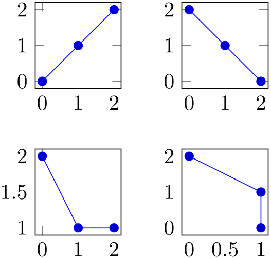

% Preamble: \pgfplotsset{width=7cm,compat=1.18}\usepgfplotslibrary{groupplots}
% Example using groupplots library
\begin{tikzpicture}
\begin{groupplot}[group style={group size=2 by 2},height=3cm,width=3cm]
\nextgroupplot
\addplot coordinates {(0,0) (1,1) (2,2)};
\nextgroupplot
\addplot coordinates {(0,2) (1,1) (2,0)};
\nextgroupplot
\addplot coordinates {(0,2) (1,1) (2,1)};
\nextgroupplot
\addplot coordinates {(0,2) (1,1) (1,0)};
\end{groupplot}
\end{tikzpicture}
\qquad
% Same example created as done without the library
\begin{tikzpicture}
\begin{axis}[name=plot1,height=3cm,width=3cm]
\addplot coordinates {(0,0) (1,1) (2,2)};
\end{axis}
\begin{axis}[name=plot2,at={($(plot1.east)+(1cm,0)$)},anchor=west,height=3cm,width=3cm]
\addplot coordinates {(0,2) (1,1) (2,0)};
\end{axis}
\begin{axis}[name=plot3,at={($(plot1.south)-(0,1cm)$)},anchor=north,height=3cm,width=3cm]
\addplot coordinates {(0,2) (1,1) (2,1)};
\end{axis}
\begin{axis}[name=plot4,at={($(plot2.south)-(0,1cm)$)},anchor=north,height=3cm,width=3cm]
\addplot coordinates {(0,2) (1,1) (1,0)};
\end{axis}
\end{tikzpicture}
The equivalent code is seen as the second example and it is clear that you have to type a lot less. So how do you use it? First of all you need to utilize the new environment groupplot. Within this environment the following command works.
-
\nextgroupplot[
axis options]
normal plot commands
This command shifts the placement of the
plot. Therefore one should always start the environment
groupplot with the command
\nextgroupplot in order to create the first plot. The
[axis options] are the options that are supplied to the following axes until the next
\nextgroupplot command is seen by
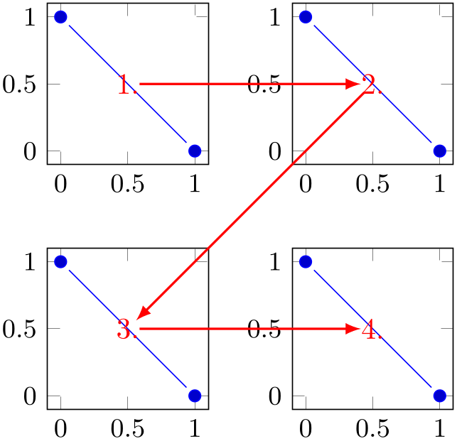
TeX. The order in which figures are typeset are as seen in the next example.
% Preamble: \pgfplotsset{width=7cm,compat=1.18}\usepgfplotslibrary{groupplots}
\begin{tikzpicture}[shorten >=4pt,shorten <=4pt]
\begin{groupplot}[group style={group size=2 by 2},
height=3.5cm,width=3.5cm,/tikz/font=\small]
\nextgroupplot% 1
\addplot coordinates {(0,1) (1,0)};
\nextgroupplot% 2
\addplot coordinates {(0,1) (1,0)};
\nextgroupplot% 3
\addplot coordinates {(0,1) (1,0)};
\nextgroupplot% 4
\addplot coordinates {(0,1) (1,0)};
\end{groupplot}
\draw [thick,>=latex,->,red]
(group c1r1.center) node {1.} --
(group c2r1.center) node {2.};
\draw [thick,>=latex,->,red]
(group c2r1.center) --
(group c1r2.center) node {3.};
\draw [thick,>=latex,->,red]
(group c1r2.center) --
(group c2r2.center) node {4.};
\end{tikzpicture}
The plot first fills the first row, then the next row and so on. Just like a table, thus the names group ccolumnrrow. The power of the groupplot is to quickly create an aligned
structure of plots. But you can also utilize it to structure data more creatively. Consider the next example.
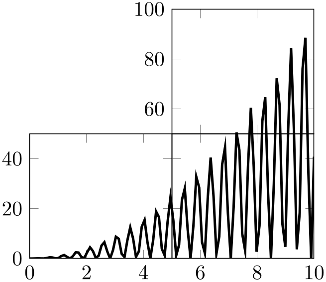
% Preamble: \pgfplotsset{width=7cm,compat=1.18}\usepgfplotslibrary{groupplots}
\begin{tikzpicture}
\begin{groupplot}[group style={group size=2 by 2,
horizontal sep=0pt,vertical sep=0pt,
xticklabels at=edge bottom},
xmin=0,ymin=0,
height=3.7cm,width=4cm,no markers]
\nextgroupplot[group/empty plot]
\nextgroupplot[xmin=5,xmax=10,ymin=50,ymax=100]
                            \addplot [very thick] file
                    {plotdata/group-1.dat};
\nextgroupplot[xmax=5,ymax=50]
                            \addplot [very thick] file
                    {plotdata/group-1.dat};
\nextgroupplot[xmin=5,xmax=10,ymax=50,yticklabels={}]
                            \addplot [very thick] file
                    {plotdata/group-1.dat};
\end{groupplot}
\end{tikzpicture}
Or for instance zooming in on data as in the next example.
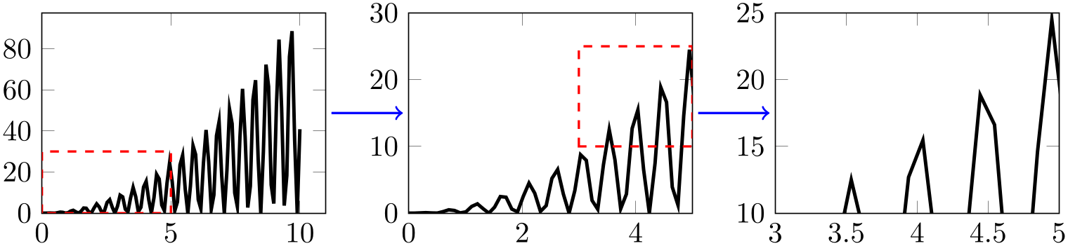
% Preamble: \pgfplotsset{width=7cm,compat=1.18}\usepgfplotslibrary{groupplots}
\begin{tikzpicture}
\begin{groupplot}[group style={group size=3 by 1},xmin=0,ymin=0,height=4cm,width=5cm,no markers]
\nextgroupplot
\addplot [very thick] file
{plotdata/group-1.dat};
\draw [red,dashed,thick] (0,0) rectangle (5,30);
\nextgroupplot[xmax=5,ymax=30]
\addplot [very thick] file
{plotdata/group-1.dat};
\draw [red,dashed,thick] (3,10) rectangle (5,25);
\nextgroupplot[xmin=3,xmax=5,ymin=10,ymax=25]
\addplot [very thick] file
{plotdata/group-1.dat};
\end{groupplot}
\draw [thick,blue,->,shorten >=2pt,shorten <=2pt]
                            (group c1r1.east) --
                    (group c2r1.west);
\draw [thick,blue,->,shorten >=2pt,shorten <=2pt]
                            (group c2r1.east) --
                    (group c3r1.west);
\end{tikzpicture}
5.8.1Grouping options
-
/pgfplots/group style={
options with group/ prefix}
This key sets all
options
using the /pgfplots/group/ prefix.
Note that the distinction between group/ and normal options is important as some of them are quite similar.
For example, the following statements are all equivalent:
\pgfplotsset{group style={a=2,b=3}}
\pgfplotsset{group/a=2,group/b=3}
\pgfplotsset{group/.cd,a=2,b=3}
All the following keys are in the subdirectory group.
-
/pgfplots/group/group size=
columns
by
rows (initially 1 by 1)
-
/pgfplots/group/columns=
columns (initially 1)
-
/pgfplots/group/rows=
rows (initially 1)
These keys determine the total
number of plots that can be in one environment groupplot. It is thus important not to add more
\nextgroupplot in the environment than
columns\(\times \)rows. This is critical to set if one uses more than 1 more plot. As the key
group size uses
columns and
rows you should stick to either
group size or both
columns and
rows.
-
/pgfplots/group/xlabels at=all|edge bottom|edge top (initially all) 
-
/pgfplots/group/ylabels at=all|edge left|edge right (initially all) 
In order to determine which plots get labels typeset one can use these keys. By default all axes get typeset normally and thus have both \(x\)- and \(y\)-axis labels.
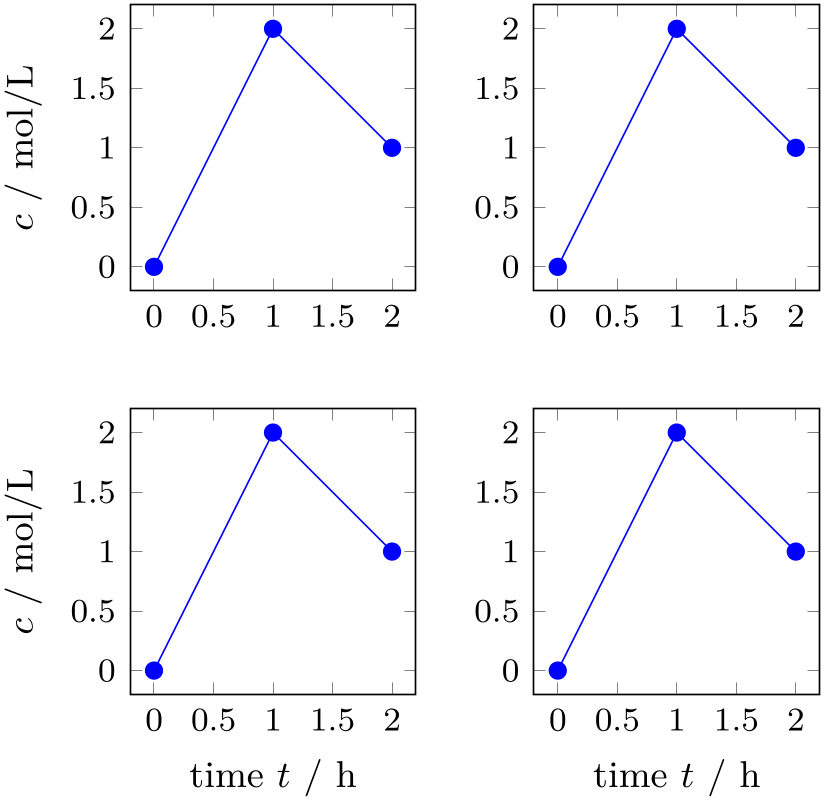
% Preamble: \pgfplotsset{width=7cm,compat=1.18}\usepgfplotslibrary{groupplots}
\begin{tikzpicture}
\begin{groupplot}[
group style={
group name=my plots,
group size=2 by 2,
xlabels at=edge bottom,
ylabels at=edge left,
},
footnotesize,
width=4cm,
height=4cm,
%
xlabel=time $t$ / h,
ylabel=$c$ / mol/L,
]
\nextgroupplot
\addplot coordinates {(0,0) (1,2) (2,1)};
\nextgroupplot
\addplot coordinates {(0,0) (1,2) (2,1)};
\nextgroupplot
\addplot coordinates {(0,0) (1,2) (2,1)};
\nextgroupplot
\addplot coordinates {(0,0) (1,2) (2,1)};
\end{groupplot}
\end{tikzpicture}
In the example above, only the bottom row gets the label defined in the beginning groupplot environment on the \(x\)-axis and only the first column of plots gets labels on the \(y\)-axis on their left side. These keys are especially handy when using glued plots.
-
/pgfplots/group/xticklabels at=all|edge top|edge bottom (initially all) 
-
/pgfplots/group/yticklabels at=all|edge left|edge right (initially all) 
In order to determine which plots get tick labels typeset one can use these keys. By default all axes gets typeset normally and thus have both \(x\)- and \(y\)-axis tick labels. If one sets
only the bottom row gets tick labels on the \(x\)-axis and only the last column gets tick labels on the \(y\)-axis on their right side. These keys are specially handy when using glued plots.
Keep in mind that this is implies the same ticks for all plots.
-
/pgfplots/group/x descriptions at=all|edge top|edge bottom (initially all) 
-
/pgfplots/group/y descriptions at=all|edge left|edge right (initially all) 
These are simply a short hand for using both xticklabels at and xlabels at simultaneously:
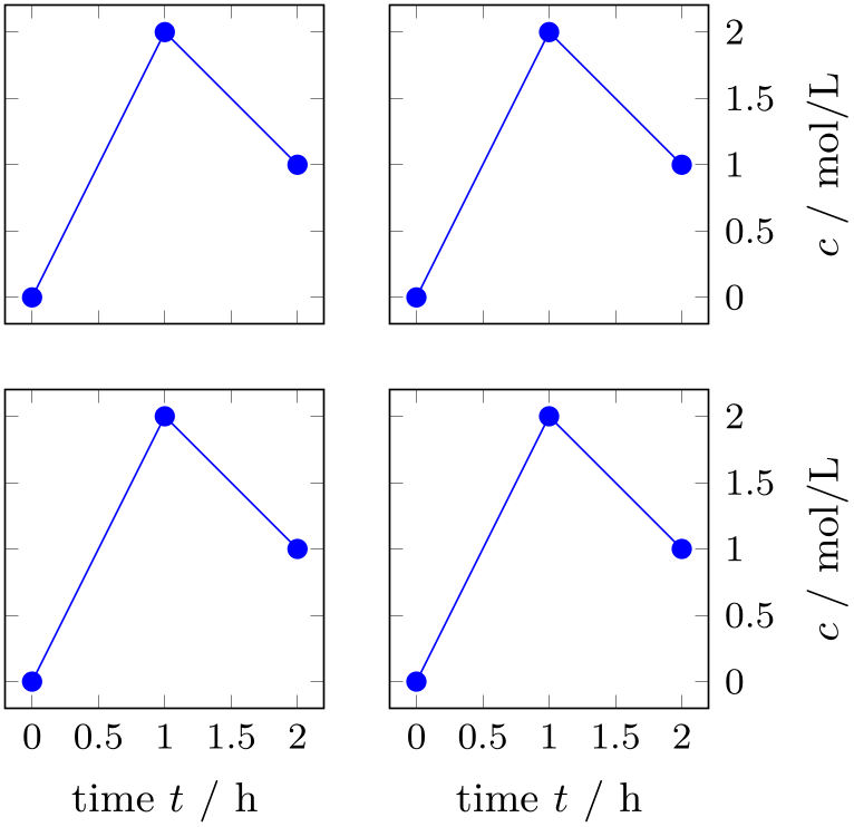
% Preamble: \pgfplotsset{width=7cm,compat=1.18}\usepgfplotslibrary{groupplots}
\begin{tikzpicture}
\begin{groupplot}[
group style={
group name=my plots,
group size=2 by 2,
%
x descriptions at=edge bottom,
y descriptions at=edge right,
horizontal sep=0.5cm,
vertical sep=0.5cm,
},
footnotesize,
width=4cm,
height=4cm,
%
xlabel=time $t$ / h,
ylabel=$c$ / mol/L,
]
\nextgroupplot
\addplot coordinates {(0,0) (1,2) (2,1)};
\nextgroupplot
\addplot coordinates {(0,0) (1,2) (2,1)};
\nextgroupplot
\addplot coordinates {(0,0) (1,2) (2,1)};
\nextgroupplot
\addplot coordinates {(0,0) (1,2) (2,1)};
\end{groupplot}
\end{tikzpicture}
Here, x descriptions at=edge bottom yields that \(x\) descriptions (xlabel and xticklabel) are only used for the lowest row. Furthermore, y descriptions at=edge right places \(y\) descriptions only for the rightmost column. Consider modifying the horizontal sep and vertical sep for your needs.
As for xticklabels at, usage of this key implies the same ticks for all plots.
This might require compat=1.3 (or newer).
-
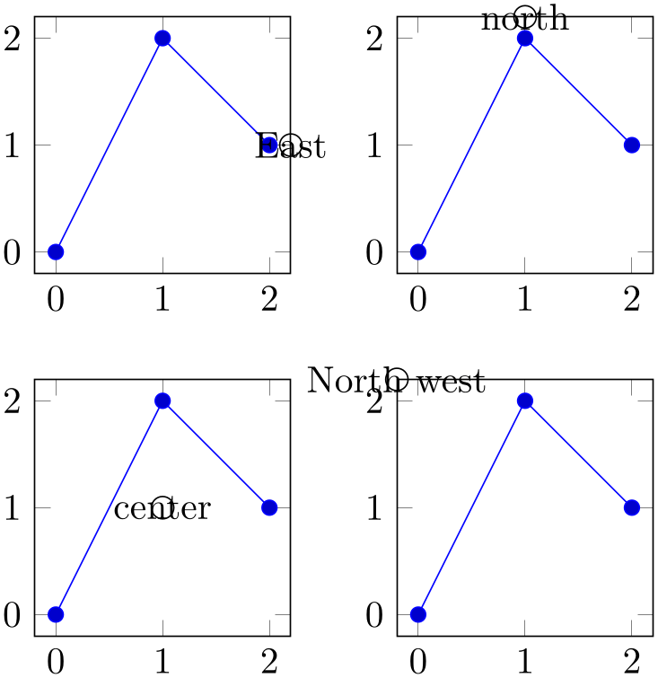
/pgfplots/group/group name={
name} (initially group)
This sets what you can refer the plots to after typesetting. Thus you can use their anchors later. See the following example
% Preamble: \pgfplotsset{width=7cm,compat=1.18}\usepgfplotslibrary{groupplots}
\begin{tikzpicture}
\begin{groupplot}[
group style={
group name=my plots,
group size=2 by 2,
},
width=4cm,height=4cm,
]
\nextgroupplot
\addplot coordinates {(0,0) (1,2) (2,1)};
\nextgroupplot
\addplot coordinates {(0,0) (1,2) (2,1)};
\nextgroupplot
\addplot coordinates {(0,0) (1,2) (2,1)};
\nextgroupplot
\addplot coordinates {(0,0) (1,2) (2,1)};
\end{groupplot}
\draw (my plots c1r1.east)
circle (3pt) node {East};
\draw (my plots c2r1.north)
circle (3pt) node {north};
\draw (my plots c1r2.center)
circle (3pt) node {center};
\draw (my plots c2r2.north west)
circle (3pt) node {North west};
\end{tikzpicture}
-
/pgfplots/group/empty plot/.style={
style} (initially /pgfplots/hide axis)
This key can be used as an option to the command \nextgroupplot. This makes the next plot invisible (only the axes) but maintains it anchors and name. If you want it to behave in another style then you can redefine it. Consider the same example as before.
% Preamble: \pgfplotsset{width=7cm,compat=1.18}\usepgfplotslibrary{groupplots}
\begin{tikzpicture}
\begin{groupplot}[
group style={
group name=my plots,
group size=2 by 2,
},
width=4cm,height=4cm,
]
\nextgroupplot[group/empty plot]
\nextgroupplot
\addplot coordinates {(0,0) (1,2) (2,1)};
\nextgroupplot
\addplot coordinates {(0,0) (1,2) (2,1)};
\nextgroupplot
\addplot coordinates {(0,0) (1,2) (2,1)};
\end{groupplot}
\draw (my plots c1r1.east)
circle (3pt) node {East};
\draw (my plots c2r1.north)
circle (3pt) node {north};
\draw (my plots c1r2.center)
circle (3pt) node {center};
\draw (my plots c2r2.north west)
circle (3pt) node {North west};
\end{tikzpicture}
Notice that you need to call a \nextgroupplot again to jump to the next plot.