Manual for Package pgfplots
2D/3D Plots in LATeX, Version 1.18.2
https://github.com/pgf-tikz/pgfplots
Related Libraries
5.9Patchplots Library
-
\usepgfplotslibrary{patchplots} % LaTeX and plain TeX 
-
\usepgfplotslibrary[patchplots] % ConTeXt 
-
\usetikzlibrary{pgfplots.patchplots} % LaTeX and plain TeX 
-
\usetikzlibrary[pgfplots.patchplots] % ConTeXt 
A library for advanced patch plots. Its strength is the creation of patches with smooth boundaries and smoothly shaded colors.
A patch plot is a plot in which each individual patch is available. Here, “available” means that the user provided each individual patch manually. This can be achieved by means of a long series of patches which have been concatenated in a suitable way (compare the description of patch plots in Section 4.6.13) or by means of a mathematical expression which is sampled (compare the key patch type sampling). Most patch types expect a series of point evaluations in a specific sequence.
Note that even though each individual patch might have a smooth boundary, the patchplots library does not interpolate smoothly between adjacent patches. Consequently, it is task of the one who creates the patches (which means: evaluated some function at its vertices) to ensure that patches can be glued together in an adequate way. This allows a lot of freedom, including both jumps and smoothly concatenated edges.
The patchplots library comes with a couple of inherently two-dimensional patch types (including second order triangles/rectangular patches and cubic tensor product patches known for finite elements). Typically, these patches live in a three-dimensional axis. Often, they are used to visualize the surface of function values \(f(x,y)\). The patchplots library ensures that such patches are drawn in a way which respects the current view. In particular, if a patch folds over itself (which is possible), it is drawn such that foreground areas are in the foreground and background areas are in the background.
The patchplots library comes with smoothly shaded patches. More precisely, both the boundary of patches and their color shading are smooth. Note, however, that the patch boundary typically has much more smoothness than the color shading.
The patchplots library also allows automatic conversion from a higher order patch to triangles (triangulation) by means of the key patch to triangles. Furthermore, it features automatic patch refines.
Use the patchplots library if you want to have smooth boundaries for your patches, or if you need advanced shadings, or if you want polygon plots, or if you want more freedom in one-dimensional patches.
5.9.1Additional Patch Types
-
/pgfplots/patch type=default|rectangle|triangle|line|quadratic spline|cubic spline|
bezier spline|bilinear|triangle quadr|biquadratic|bicubic|polygon|coons|tensor bezier (initially default)
The patchplots library supports several new patch types in addition to the initially available choices (which are rectangle,triangle and line). The documentation of the two-dimensional choices from page (page for section 4.6.13) is repeated here.
The new patch types are discussed in detail on the following pages.
5.9.1.1One-Dimensional Patch Types
There are three new one-dimensional patch types, namely quadratic spline, cubic spline, and bezier spline. Here, patch type=quadratic spline consists of quadratic patches of \(n=3\) vertices each. The vertices are interpolated exactly:
% Preamble: \pgfplotsset{width=7cm,compat=1.18}\usepgfplotslibrary{patchplots}
\begin{tikzpicture}
\begin{axis}[
nodes near coords={(\coordindex)},
                      title={\texttt{patch
                  type=quadratic spline}},
]
\addplot [
mark=*,
patch,
patch type=quadratic spline,
] coordinates {
% left, right, middle-> first segment
(0,0) (1,1) (0.5,0.5^2)
% left, right, middle-> second segment
(1.2,1) (2.2,1) (1.7,2)
};
\end{axis}
\end{tikzpicture}
In our example, the first segment interpolates \(f(x)=x^2\) at the points \(\{0,\nicefrac 12,1\}\). The quadratic spline is actually nothing but piecewise Lagrangian interpolation with quadratic polynomials: it expects three points in the sequence ‘(left end), (right end), (middle)’ and interpolates these three points with a quadratic polynomial. Unlike the default 1d mesh visualization (which uses patch type=line implicitly), you have to use the special syntax above (or the equivalent approach by means of patch table). Note that patch type=quadratic spline results in correct shapes, but uses just constant color for each segment; high order color shading is only supported approximately using patch refines.
The patch type=cubic spline is very similar: it expects patches of \(n=4\) vertices and interpolates them with a cubic polynomial:
% Preamble: \pgfplotsset{width=7cm,compat=1.18}\usepgfplotslibrary{patchplots}
\begin{tikzpicture}
\begin{axis}[
nodes near coords={(\coordindex)},
                      title={\texttt{patch type=cubic
                  spline}},
]
\addplot [
mark=*,
patch,
patch type=cubic spline,
] coordinates {
% left, right, left middle, right middle
(-1,-1)
(1,1)
(-1/3,{(-1/3)^3})
(1/3,{(1/3)^3})
};
\end{axis}
\end{tikzpicture}
Here, we interpolated \(f(x)=x^3\) at the four equidistant points \(\{-1,-\nicefrac 13,\nicefrac 13,1\}\) with a cubic polynomial (which is \(x^3\)). The cubic spline expects a sequence of patches, each with four coordinates, given in the sequence ‘(left end), (right end), (interpolation point at \(\nicefrac 13\)), (interpolation point at \(\nicefrac 23\))’. It has limitations and features like quadratic spline, see above.
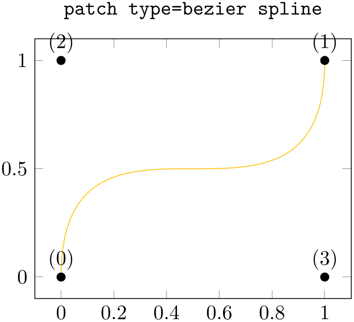
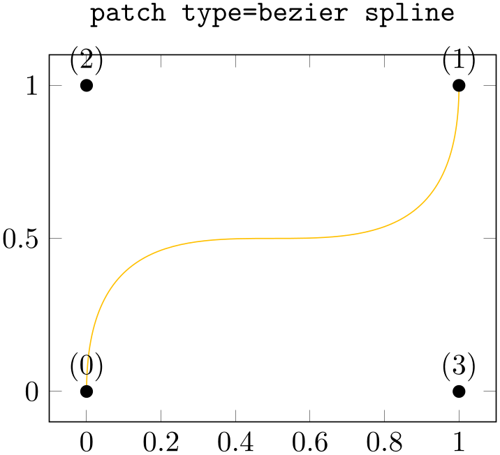
Finally, patch type=bezier spline is the same as if you provide a couple of TikZ drawing instructions with curveto operations: it expects a sequence of \(n=4\) vertices in the order left endpoint, right endpoint, first control point, second control point. Consequently, it is different from most other patch types listed in this section:
% Preamble: \pgfplotsset{width=7cm,compat=1.18}\usepgfplotslibrary{patchplots}
\begin{tikzpicture}
\begin{axis}[
nodes near coords={(\coordindex)},
                      title={\texttt{patch type=bezier
                  spline}},
]
\addplot [
mark=*,
patch,
patch type=bezier spline,
] table {
% left, right, first control, second control
0 0
1 1
0 1
1 0
};
\end{axis}
\end{tikzpicture}
the patch type bezier spline currently supports no patch refines, no patch type sampling, and has an inaccurate bounding box. Its primary use is to serve as input to other tools which generate bezier splines or as limited drawing tool which is integrated into pgfplots.
5.9.1.2Providing Patches by means of Mathematical Expressions
Most patch types expect a specific number of vertices in a specific sequence. This is part of what the patchplots library is. But is is still tedious to provide this sort of data.
For simple patch types like line,rectangle and bilinear, you can provide the input coordinates with any of the input methods which are available for all other plot handlers. In particular, line is just a sharp plot (with individually colored segments) and rectangle is nothing but a surf plot. Note that both rectangle and bilinear also accept the standard matrix input (with scanlines, see mesh/ordering and its documentation). In summary: simple patch types accept a simple input format.
-
/pgfplots/patch type sampling=true|false (initially false) 
There are some complicated patch types. In particular, all patch types of higher order (i.e. quadratic spline, cubic spline, triangle quadr, biquadratic, bicubic) need more points than just their corners. For such patch types, you need to resort to mesh input=patches. That means you need to provide extra vertices and their function evaluation values in a specific sequence.
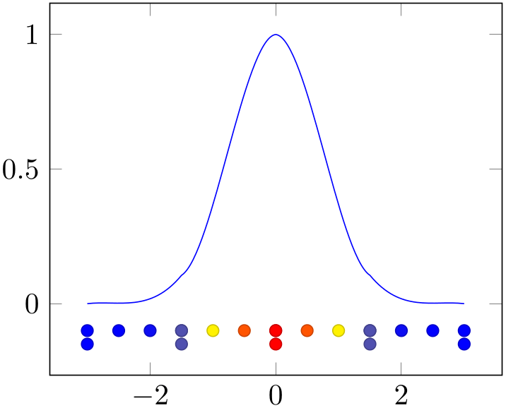
The patch type sampling method allows to simplify the procedure for such complicated patch types:91 it works together with \addplot expression and evaluates the mathematical expression at each of the required vertices (in the correct sequence):

% Preamble: \pgfplotsset{width=7cm,compat=1.18}\usepgfplotslibrary{patchplots}
\begin{tikzpicture}
\begin{axis}
\addplot [
samples=5,domain=-3:3,
mesh,patch type=cubic spline,
patch type sampling,
% avoid individual colors per segment:
blue,point meta=none,
]
{exp(-x^2)};
% a second plot which shows the
% generated x positions:
\addplot [
mark=*,only marks,scatter,
samples=5,domain=-3:3,
patch type=cubic spline,
patch type sampling,
point meta={exp(-x^2)},
]
{-0.1};
% a third plot which shows the marks
% without patch type sampling:
\addplot [
mark=*,only marks,scatter,
samples=5,domain=-3:3,
point meta={exp(-x^2)},
]
{-0.15};
\end{axis}
\end{tikzpicture}
The first plot above is almost a normal plot by expression. The samples and domain key controls the sampling procedure, and blue,point meta=none defines the global color to use. Note that the special choice point meta=none simply disables individual colors per mesh segment (which is the default for mesh plots). However, the patch type sampling key here makes a huge difference: it tells pgfplots to check the current value of patch type and to sample a coordinate sequence which is suitable as input for that patch type. We see that the outcome is a partially smooth function (more about that below).
The method patch type sampling samples x just as usual. The result is a sequence \([x_0,x_1,\dotsc ,x_k]\). For each interval \([x_i,x_{i+1}]\), a patch type is sampled inside of the interval. To this end, the current patch type is used to generate a standardized vertex pattern in the unit cube. For patch type=cubic spline, this generates four points \(0, \nicefrac 13, \nicefrac 23, 1\). These standardized numbers are mapped into \([x_i, x_{i+1}]\). Then, any mathematical expressions (in our case exp(-x^2)) are evaluated at the resulting positions.
The second plot in our example above shows the markers resulting from patch type sampling. Note that we see \(13\) markers even though we have said samples=5. These \(5\) samples are shown in the third plot. This is because patch type=cubic spline needs \(4\) points for each patch (i.e. \(4\) points in each sampled interval).
Note that even though the result in our example above is partially smooth, it is not globally smooth. In other words: each resulting mesh segment is a polynomial of third order. But: the five cubic polynomials are determined independently; and they are simple glued together without any intelligence. In particular, they are unsmooth at the five initial sampling points! This key cannot apply global smoothing. It is really just a convenient method which simplifies sampling of such patch types.
The method patch type sampling can also be used for surf plots, i.e. for matrix sampling. It works in the same way:

% Preamble: \pgfplotsset{width=7cm,compat=1.18}\usepgfplotslibrary{patchplots}
\begin{tikzpicture}
\begin{axis}
\addplot3 [surf,shader=interp,
patch type=bicubic,
patch type sampling,
samples=5,domain=-3:3,
] {exp(-x^2-y^2)};
% show the generated grid on top:
\addplot3 [
mark=*,mark size=1pt,only marks,scatter,
samples=5,domain=-3:3,
patch type=bicubic,
patch type sampling,
point meta={exp(-x^2-y^2)},
] {1.1};
\end{axis}
\end{tikzpicture}
The example is similar to our one-dimensional example above: it uses the same 1d function as product. We see that it has \(13^2\) samples instead of just \(5^2\), and we see that the geometry is partially smooth (see above for “partially”). Note, however, that the color interpolation is only applied once per patch. The following example shows a bilinear patch with unsmooth geometry, but higher resolution for the color data, on a \(13\times 13\) mesh:
% Preamble: \pgfplotsset{width=7cm,compat=1.18}\usepgfplotslibrary{patchplots}
\begin{tikzpicture}
\begin{axis}
\addplot3 [surf,shader=interp,
patch type=bilinear,
samples=13,domain=-3:3,
] {exp(-x^2-y^2)};
% show the generated grid on top:
\addplot3 [
mark=*,mark size=1pt,only marks,scatter,
samples=13,domain=-3:3,
point meta={exp(-x^2-y^2)},
] {1.1};
\end{axis}
\end{tikzpicture}
Note that you may want to view the preceding examples in Acrobat Reader. Many free PDF viewers cannot display these shadings properly.
5.9.1.3Global One-Dimensional Curves with Smooth Splines
Typically, pgfplots assumes that you want individually colored patch segments whenever you use one of the plot handlers mesh, surf, or patch. The individual colors are determined by the current colormap and the value of point meta (compare Section 4.8).
Technically, individually colored path segments are one unit. If you fill them, you fill only one segment. You cannot fill them against the axis. In particular, you cannot use \closedcycle for individually colored mesh or patch plots.
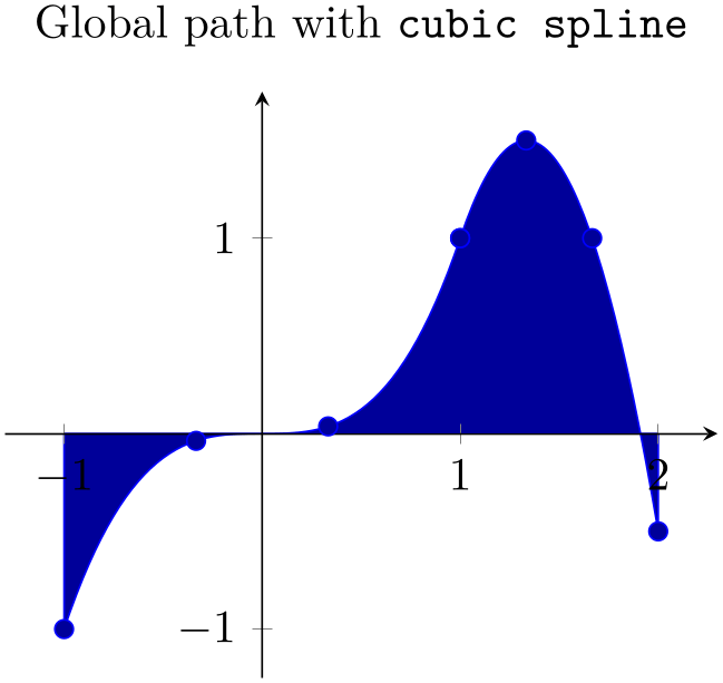
The patchplots library comes with one-dimensional patch types like quadratic spline or cubic spline. It would be useful to draw a global path, that is: one which has a single color such that \closedcycle works. This is supported if you write point meta=none:
% Preamble: \pgfplotsset{width=7cm,compat=1.18}\usepgfplotslibrary{patchplots}
\begin{tikzpicture}
\begin{axis}[
axis lines=middle,
axis on top,
enlargelimits,
                      title={Global path with
                  \texttt{cubic spline}},
]
\addplot [
mark=*,
patch,
patch type=cubic spline,
point meta=none,% allow \closedcycle
blue,
fill=blue!60!black,
] table {
% left, right, left middle, right middle
                          -1
                           -1
                          1
                            1
-0.333333 -0.037037
0.333333 +0.037037
                          1
                            1
                          2
                            -0.5
1.333333 1.5
1.666666 1
}
\closedcycle;
\end{axis}
\end{tikzpicture}
The use of point meta=none activates a special processing: the outcome is precisely one path.
5.9.1.4Two-Dimensional Patch Types
The patchplots library is especially strong for shader=interp, so this is our main focus in the remaining documentation here.
At the time of this writing, many free PDF viewers do not fully support the following shadings.92 The preferred viewer is Adobe Acrobat Reader.
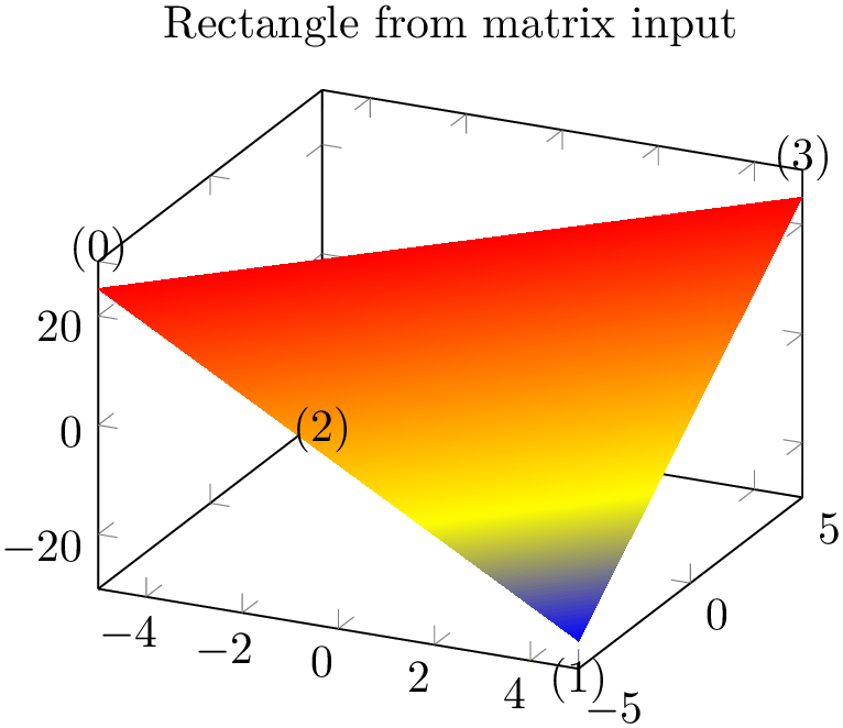
The choice rectangle expects one or more rectangular patches with \(n=4\) vertices each. These vertices are either encoded as a matrix or as individual patches (using mesh input=patches), in the sequence in which you would connect the vertices:
% Preamble: \pgfplotsset{width=7cm,compat=1.18}\usepgfplotslibrary{patchplots}
\begin{tikzpicture}
\begin{axis}[
nodes near coords={(\coordindex)},
                      title=Rectangle from matrix
                  input,
]
% note that surf implies 'patch type=rectangle'
\addplot3 [
surf,
shader=interp,
samples=2,
patch type=rectangle,
] {x*y};
\end{axis}
\end{tikzpicture}
% Preamble: \pgfplotsset{width=7cm,compat=1.18}\usepgfplotslibrary{patchplots}
\begin{tikzpicture}
\begin{axis}[
nodes near coords={(\coordindex)},
title=Rectangle from patch input,
]
\addplot3 [
patch,
shader=interp,
patch type=rectangle,
] coordinates {
(0,0,1) (1,0,0) (1,1,0) (0,1,0)
};
\end{axis}
\end{tikzpicture}
As already documented on page (page for section 4.6.13), the shader=interp implementation for rectangle uses two triangles and interpolates them linearly. The differences between the two examples above arise due to \(z\) buffering approaches: the matrix input reorders the matrix in linear time, whereas the second example would sort complete rectangles. In our case, this yields to the different corner sequence.
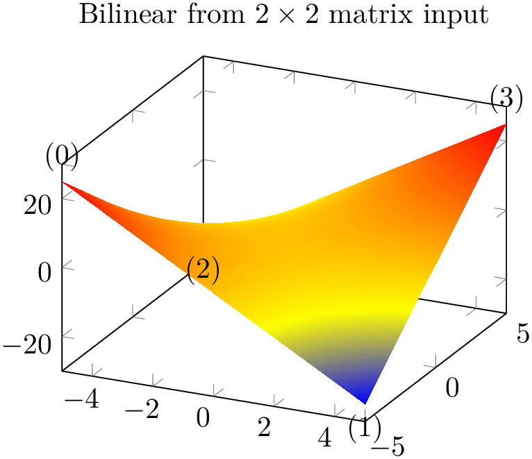
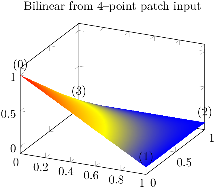
The choice bilinear is essentially the same as rectangular with respect to its input formats and stroke paths, but it uses correct bilinear shading for shader=interp. Moreover, the geometry is also interpolated bilinearly instead of just two triangles. The two examples from above now become
% Preamble: \pgfplotsset{width=7cm,compat=1.18}\usepgfplotslibrary{patchplots}
\begin{tikzpicture}
\begin{axis}[
nodes near coords={(\coordindex)},
                      title=Bilinear from
                  $2\times 2$ matrix input,
]
% note that surf implies 'patch type=rectangle'
\addplot3 [
surf,
shader=interp,
samples=2,
patch type=bilinear,
] {x*y};
\end{axis}
\end{tikzpicture}
% Preamble: \pgfplotsset{width=7cm,compat=1.18}\usepgfplotslibrary{patchplots}
\begin{tikzpicture}
\begin{axis}[
nodes near coords={(\coordindex)},
                      title=Bilinear from $4$--point
                  patch input,
]
\addplot3 [
patch,
shader=interp,
patch type=bilinear,
] coordinates {
(0,0,1) (1,0,0) (1,1,0) (0,1,0)
};
\end{axis}
\end{tikzpicture}
Use patch type=bilinear if you want to improve the shape of individual patches and the quality of the color interpolation. In contrast to the simpler patch type=rectangle, it might result in a huger output document.
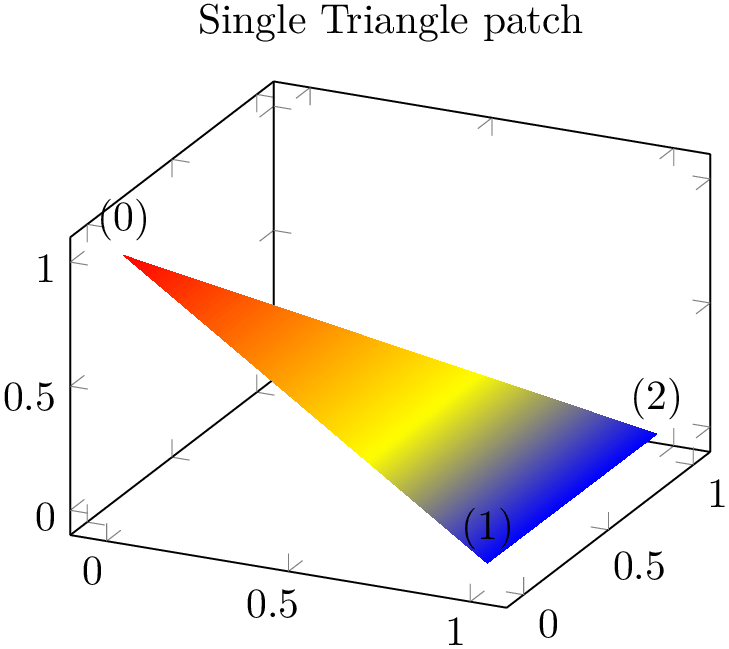
The choice triangle expects a sequence of linear triangles, each encoded using \(n=3\) vertices:
% Preamble: \pgfplotsset{width=7cm,compat=1.18}\usepgfplotslibrary{patchplots}
\begin{tikzpicture}
\begin{axis}[
enlargelimits,
nodes near coords={(\coordindex)},
title=Single Triangle patch,
]
\addplot3 [
patch,
shader=interp,
] coordinates {
(0,0,1)
(1,0,0)
(1,1,0)
};
\end{axis}
\end{tikzpicture}
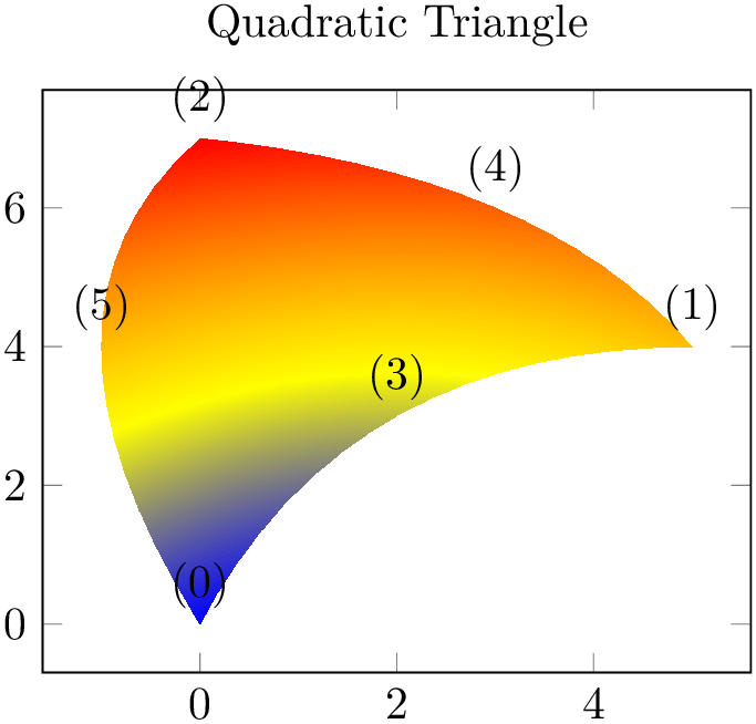
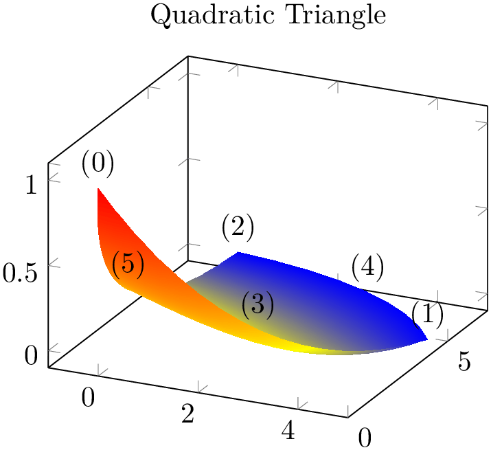
The choice triangle quadr expects a sequence of isoparametric quadratic triangles, each defined by \(n=6\) vertices:

% Preamble: \pgfplotsset{width=7cm,compat=1.18}\usepgfplotslibrary{patchplots}
\begin{tikzpicture}
\begin{axis}[
nodes near coords={(\coordindex)},
title=Quadratic Triangle,
]
\addplot [
patch,
patch type=triangle quadr,
shader=interp,
point meta=explicit,
] coordinates {
(0,0) [1] (5,4) [2] (0,7) [3]
(2,3) [1] (3,6) [2] (-1,4) [3]
};
\end{axis}
\end{tikzpicture}

% Preamble: \pgfplotsset{width=7cm,compat=1.18}\usepgfplotslibrary{patchplots}
\begin{tikzpicture}
\begin{axis}[
nodes near coords={(\coordindex)},
title=Quadratic Triangle,
]
\addplot3 [
patch,
patch type=triangle quadr,
shader=interp,
] coordinates {
(0,0,1) (5,4,0) (0,7,0)
(2,3,0) (3,6,0) (-1,4,0)
};
\end{axis}
\end{tikzpicture}
Here, the edges have the correct quadratic shape. However, the color interpolation is just bilinear; using the color values of the corners and ignoring the rest (consider using patch refines to improve the color interpolation). For three dimensions, pgfplots checks the depth of corners to determine foreground/background. For two dimensions, strongly distorted elements may fold over each other in unexpected ways.
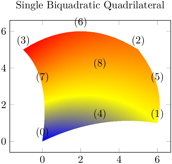
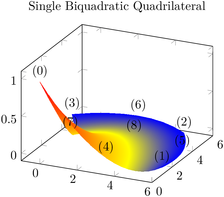
The choice biquadratic expects a sequence of isoparametric biquadratic quadrilaterals each defined by \(n=9\) vertices. Their main use is to get “rectangles” with smooth boundaries:
% Preamble: \pgfplotsset{width=7cm,compat=1.18}\usepgfplotslibrary{patchplots}
\begin{tikzpicture}
\begin{axis}[
nodes near coords={(\coordindex)},
                      title=Single Biquadratic
                  Quadrilateral,
]
\addplot [
patch,
patch type=biquadratic,
shader=interp,
point meta=explicit,
] coordinates {
(0,0) [1] (6,1) [2] (5,5) [3] (-1,5) [4]
(3,1) [1] (6,3) [2] (2,6) [3] (0,3) [4]
(3,3.75) [4]
};
\end{axis}
\end{tikzpicture}
% Preamble: \pgfplotsset{width=7cm,compat=1.18}\usepgfplotslibrary{patchplots}
\begin{tikzpicture}
\begin{axis}[
nodes near coords={(\coordindex)},
                      title=Single Biquadratic
                  Quadrilateral,
]
\addplot3 [
patch,
patch type=biquadratic,
shader=interp,
] coordinates {
(0,0,1) (6,1,0) (5,5,0) (-1,5,0)
(3,1,0) (6,3,0) (2,6,0) (0,3,0)
(3,3.75,0)
};
\end{axis}
\end{tikzpicture}
Similar to triangle quadr, the edges have the correct quadratic shape – but the color interpolation is just bilinear; using the color values of the corners and ignoring the rest. Again, ensure that the mesh width is small enough in order to improve the quality of the color interpolation (see also patch refines).
Note that a function of \((x,y)\) is biquadratic if it is quadratic w.r.t. \(x\) if \(y=\text {const}\) and also
quadratic w.r.t. \(y\) if \(x=\text {const}\) (note that this is not an “if and only if”). For example,
\(f(x,y) = x^2-y^2\) is biquadratic. Consequently, we can represent a surface plot of \(f\) with just one biquadratic patch
– only the color interpolation is just bilinear. We do so using
\addplot table[z expr= expression
 ]:
]:
% Preamble: \pgfplotsset{width=7cm,compat=1.18}\usepgfplotslibrary{patchplots}
\begin{tikzpicture}
\begin{axis}
\addplot3 [patch,patch refines=3,
                          shader=faceted
                  interp,
patch type=biquadratic,
] table [z expr=x^2-y^2] {
x y
-2 -2
2 -2
2 2
-2 2
0 -2
2 0
0 2
-2 0
0 0
};
\end{axis}
\end{tikzpicture}
We see that the shape’s boundary is reconstructed exactly using the biquadratic patch. In addition, patch refines improves the (first order) color interpolation. Details for patch refines are discussed in Section 5.9.2 and details and limitations regarding superimposed grid lines are discussed in Section 5.9.4.
Note that biquadratic can easily be combined with patch type sampling in order to sample an arbitrary surface plot with smooth boundaries.
A patch with type biquadratic and shader=interp has a bounding box which is determined from the input vertices. Due to the high order of the patch, parts of the patch can be outside of that bounding box. This holds for all advanced patch types.
The choice bicubic is similar to biquadratic: it allows to defines two-dimensional patches whose boundary is defined by four cubic polynomials. Consequently, it allows very smooth boundaries – especially since the viewer constructs these boundaries at every zoom level. A bicubic patch is constructed from \(16\) points which are arranged in a \(4\times 4\) matrix. Each consecutive \(16\) points make up a single bicubic patch. The \(17\)th point starts the next bicubic patch (just as for any other patch type).

% Preamble: \pgfplotsset{width=7cm,compat=1.18}\usepgfplotslibrary{patchplots}
\begin{tikzpicture}
\begin{axis}[
nodes near coords={(\coordindex)},
                      title=Single Bicubic
                  Quadrilateral,
]
\addplot3 [
patch,
patch type=bicubic,
shader=interp,
] coordinates {
(0,0,1) (1,0,0) (2,0,0) (3,0,0)
(0,1,0) (1,1,0) (2,1,0) (3,1,0)
(0,2,0) (1,2,0) (2,2,0) (3,2,0)
(0,3,0) (1,3,0) (2,3,0) (3,3,0)
};
\end{axis}
\end{tikzpicture}
Just as for biquadratic, the color interpolation of bicubic is (just) bilinear, even though the geometry is of higher order. The color interpolation uses the point meta values determined at the four corners of each patch; all other values of point meta are ignored by the shader (although their values are used to compute point meta min and point meta max).

% Preamble: \pgfplotsset{width=7cm,compat=1.18}\usepgfplotslibrary{patchplots}
\begin{tikzpicture}
                  \begin{axis}[title=Two
                  Bicubic Patches]
\addplot3 [patch,patch type=bicubic,
shader=interp,point meta=explicit,
                          ] coordinates
                  {
(0,0,1)[1] (1,0,0)[0] (2,0,0)[0] (3,0,0)[0]
(0,1,0)[0] (1,1,0)[0] (2,1,0)[0] (3,1,0)[0]
(0,2,0)[0] (1,2,0)[0] (2,2,0)[0] (3,2,0)[0]
(0,3,0)[0] (1,3,0)[0] (2,3,0)[0] (3,3,0)[0]
(3,0,0)[0] (4,0,0)[0] (5,0,0)[0] (6,0,0)[0.7]
(3,1,0)[0] (4,1,.5)[1](5,1,0)[0] (6,1,0)[0]
(3,2,0)[0] (4,2,0)[0] (5,2,0)[0] (6,2,0)[0]
(3,3,0)[0] (4,3,0)[0] (5,3,0)[0] (6,3,0)[0.1]
};
\end{axis}
\end{tikzpicture}
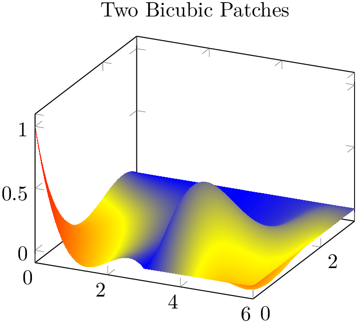
The previous example uses two patches of type bicubic. Note that the color data (point meta) has been provided explicitly – and its values are only used at the corners (the [1] value after the point (4,1,.5) is ignored). Color interpolation of bicubic patches uses only the color data at the patch’s corners. The remaining color data values are ignored. Note that if you leave the default (which is point meta=f(x) instead of point meta=explicit), the second patch will be blue. This is because the four corner vertices of the second patch define the color shading – and their \(z\) value is \(0\).
Note that bicubic can easily be combined with patch type sampling in order to sample an arbitrary surface plot with smooth boundaries.
Just as described for biquadratic, a patch with type bicubic and shader=interp can have a bounding box which is slightly smaller than the region which is actually drawn (because the bounding box is computed from the input points).
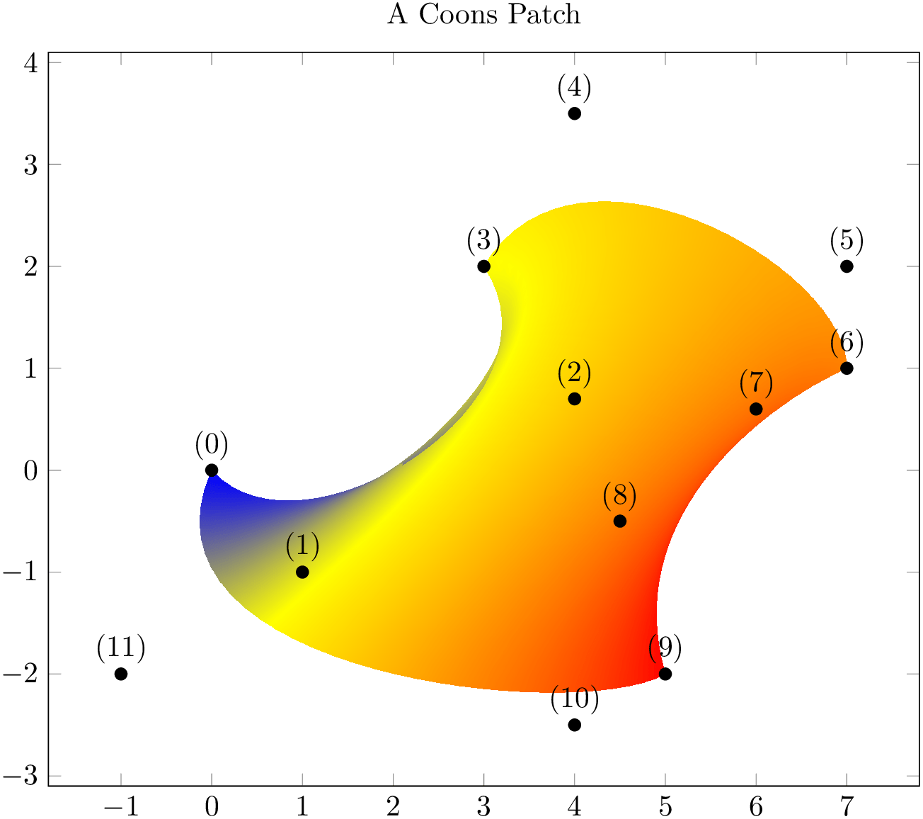
The choice coons expects a sequence of one or more Coons patches, made up of \(n=12\) points each. A Coons patch is delimited by four cubic Bézier curves, with the end points attached to each other – and the \(n\) points provide the required control points for these curves in a specific ordering which is illustrated in the following example:
% Preamble: \pgfplotsset{width=7cm,compat=1.18}\usepgfplotslibrary{patchplots}
\begin{tikzpicture}
\begin{axis}[
nodes near coords={(\coordindex)},
width=12cm,
title=A Coons Patch,
]
\addplot [mark=*,patch,patch type=coons,
shader=interp,point meta=explicit,
] coordinates
{
                              (0,0)      [0] %
                  first corner
                              (1,-1)     [0] %
                  Bezier control point between (0) and (3)
                              (4,0.7)    [0] %
                  Bezier control point between (0) and (3)
%
                              (3,2)      [1] %
                  second corner
                              (4,3.5)    [1] %
                  Bezier control point between (3) and (6)
                              (7,2)      [1] %
                  Bezier control point between (3) and (6)
%
                              (7,1)      [2] %
                  third corner
                              (6,0.6)    [2] %
                  Bezier control point between (6) and (9)
                              (4.5,-0.5) [2] % Bezier
                  control point between (6) and (9)
%
                              (5,-2)     [3] %
                  fourth corner
                              (4,-2.5)   [3] %
                  Bezier control point between (9) and (0)
                              (-1,-2)    [3] %
                  Bezier control point between (9) and (0)
};
\end{axis}
\end{tikzpicture}
The four cubic Bézier curves are equivalent to curveto paths of pgf,
i.e. to a sequence of the form ( corner 1
 ) .. controls (
 control point A
 ) and (
 control point B
 ) .. (
 corner 2
 ). The interpolated shading is bilinear. More precisely, a bilinear shading in the unit cube \([0,1]^2\) is initialised which
is then mapped into the Coons patch such that the corners match. The color interpolation uses only the color data of the four
corners, color values of intermediate control points are ignored for the shading (although their value will be respected for
the upper and lower limit of color data). In contrast to the finite element patches, a Coons patch is inherently
two-dimensional. While you can still use three-dimensional coordinates, pgfplots will draw the
shading as you provide it, without checking for the depth information (as it does for the other
patch types). In other words: depending on the current
view angle, the shading might fold over itself in
unexpected ways.
Even for two dimensions, Coons patches may fold over themselves. To determine which part is foreground and which part is background, the following rule applies: the four corner points \((0)\), \((3)\), \((6)\), \((9)\) are associated to the unit cube points \((u,v) = (0,0)\), \((0,1)\), \((1,1)\) and \((1,0)\), respectively. The edge between corner \((3)\) and \((6)\) (i.e. the one with \(v=1\)) is foreground, the edge between \((1)\) and \((9)\) is background. Thus, large values of \(v\) are drawn on top of small values of \(v\). If \(v\) is constant, large values of \(u\) are drawn on top of small values of \(u\). Thus, reordering the patch vertices (choosing a different first vertex and/or reversing the sequence) allows to get different foreground/background configurations.93
Note that patch type sampling is unavailable for patch type=coons because the control points are no point evaluation of the same function.
The choice tensor bezier is similar to patch type=coons: it allows to define a bezier patch. However, it allows more freedom: it has \(16\) control points instead of the \(12\) of a coons patch. The four additional control points are situated in the center of each patch. This patch type generates .pdf shadings of type \(7\) (whereas coons patches are shadings of type \(6\)). It has been added for reasons of completeness, although it has not been tested properly. Please refer to the specification of the .pdf format for details.94 The choice tensor bezier is actually the same as patch type=bicubic – except that bicubic automatically respects the view depth (foreground/background) and is given in a different by means of function evaluations rather than control points.
Note that patch type sampling is unavailable for patch type=tensor bezier because the control points are no point evaluation of the same function.
The choice polygon expects polygons with a fixed number of vertices. This patch type requires the number of vertices as argument:
-
/pgfplots/vertex count=
 count
count 
The number of vertices to be used for patch type=polygon. The number can be arbitrary. All input patches are expected to have this many vertices – but it is acceptable if a patch uses the same vertex multiple times. This means that patch type=polygon accepts polygons with different numbers of vertices, but you need to apply some sort of “manual padding”.
This parameter is (currently) mandatory.
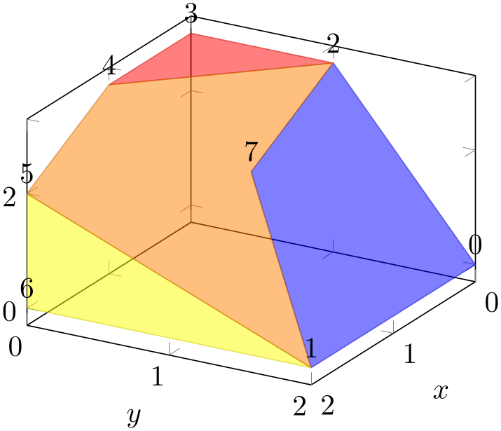
A patch plot with patch type=polygon simply connects the \(n\)=vertex count vertices in their order of appearance and closes the resulting path:
% Preamble: \pgfplotsset{width=7cm,compat=1.18}\usepgfplotslibrary{patchplots}
\begin{tikzpicture}
\begin{axis}[view/h=120,xlabel=$x$,ylabel=$y$]
\addplot3 [
opacity=0.5,
table/row sep=\\,
patch,
patch type=polygon,
vertex count=5,
patch table with point meta={
% pt1 pt2 pt3 pt4 pt5 cdata
0 1 7 2 2 0\\
1 6 5 5 5 1\\
1 5 4 2 7 2\\
2 4 3 3 3 3\\
},
] table {
                          x
                  y z\\
0 2 0\\% 0
2 2 0\\% 1
0 1 3\\% 2
0 0 3\\% 3
1 0 3\\% 4
2 0 2\\% 5
2 0 0\\% 6
1 1 2\\% 7
};
% replicate the vertex list to show \coordindex:
\addplot3 [only marks,
nodes near coords=\coordindex,
] table [row sep=\\] {
0 2 0\\ 2 2 0\\ 0 1 3\\ 0 0 3\\
1 0 3\\ 2 0 2\\ 2 0 0\\ 1 1 2\\
};
\end{axis}
\end{tikzpicture}
The example above defines the patch by means of a connectivity table (patch table with point meta) and a vertex list (the normal input coordinates of the plot): there are \(8\) vertices and \(4\) polygons. Note that \(2\) of these polygons are triangles, one has \(4\) corners and only of them actually has all \(5\) allocated corners. This effect can be achieved by replicating one of the corners. The connectivity table in our example defines a unique color for each polygon: \(0\) for the first patch, \(1\) for the second, \(2\) for the third, and \(3\) for the last. These numbers map into the current colormap.
The patch type=polygon supports neither triangulation nor shading nor refinement. The order of appearance of the input points is supposed to be the order in which the line-to operations of the resulting path are generated.
92 The author of this package has submitted bugfixes to Linux viewers based on xpdf/libpoppler, so the problem will (hopefully) vanish in future versions.
93 Internally, pgfplots employs such mechanisms to map the higher order isoparametric patch types to Coons patches, sorting according their corner’s depth information.
94 If someone is willing to test it and document it, feel free to email me!
5.9.2Automatic Patch Refinement and Triangulation
pgfplots supports automatic patch refinement for most of its patch types. There are mainly two purposes for patch refinement: to increase the quality of z buffer=sort and/or to improve color interpolation for high order patches.
-
/pgfplots/patch refines={
 levels
 } (initially 0)
This key controls patch refinement. The initial choice patch refines=0 disables refinement and visualizes elements as they have been found in input files.
A positive
 levels
 enables (recursive) patch refinement: each patch is refined individually.
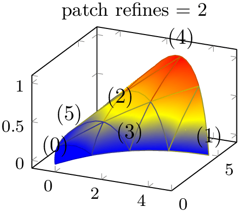
The following example illustrates the
patch refines feature for a
triangle quadr shape function on an edge. Note that since
pgfplots uses only first order shading which is based on the corner points \((0)\), \((1)\)
and \((2)\), the specified shape function of
patch refines=0 has constant color. Higher
 levels
 approximate the patch with increasing quality:
% Preamble: \pgfplotsset{width=7cm,compat=1.18}\usepgfplotslibrary{patchplots}
\foreach \level in {0,1,2} {%
\begin{tikzpicture}
\begin{axis}[
nodes near coords={(\coordindex)},
footnotesize,
title={patch refines = \level},
]
\addplot3 [patch,patch type=triangle quadr,
shader=faceted interp,patch refines=\level,
                                  ] coordinates
                      {
(0,0,0) (5,4,0) (0,7,0)
(2,3,0) (3,6,1) (-1,4,0)
};
\end{axis}
\end{tikzpicture}
}
In this example, patch refinement makes a huge difference since it is just one element with huge displacements. For practical examples, you probably won’t need many refinement levels.
The refined patches reproduce the geometry’s shape exactly. In addition, they improve color interpolation. Note that its purpose is just visualization, therefore hanging nodes are allowed (and will be generated by patch refines for most patch types).
Patch refinement is implemented for all supported patches except for patch type=coons, tensor bezier, bicubic (might follow eventually) and polygon.
-
/pgfplots/patch to triangles=true|false (initially false) 
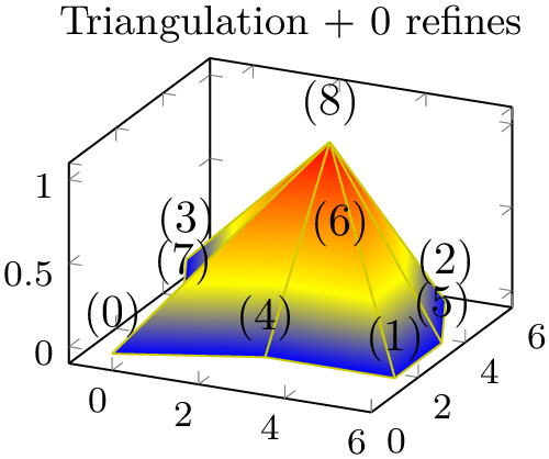
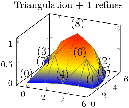
Occasionally, one has a complicated patch type on input and would like to visualize it as a triangle mesh. pgfplots supports automatic triangulation of patches. Triangulation means to replace each individual input patch by one or more triangles. Triangulation can be combined with patch refines in which case patch refines is applied first and the resulting refined patches are then triangulated.
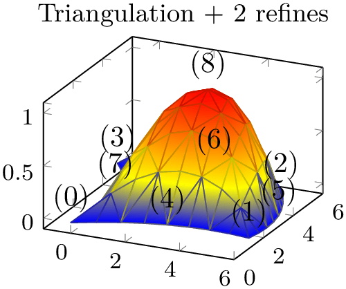


% Preamble: \pgfplotsset{width=7cm,compat=1.18}\usepgfplotslibrary{patchplots}
\foreach \level in {0,1,2} {%
\begin{tikzpicture}
\begin{axis}[
nodes near coords={(\coordindex)},
footnotesize,
title={Triangulation + \level\ refines},
]
\addplot3 [patch,patch type=biquadratic,shader=faceted interp,
patch to triangles,patch refines=\level,
                                  ] coordinates
                      {
(0,0,0) (6,1,0) (5,5,0) (-1,5,0)
(3,1,0) (6,3,0) (2,6,0) (0,3,0)
(3,3.75,1)
};
\end{axis}
\end{tikzpicture}%
}
For one-dimensional patch types like quadratic spline, patch to triangles results in approximation by means of patch type=line instead of triangle.
The patch to triangles feature is implemented for all supported patches except for patch type=coons, tensor bezier, and polygon.
5.9.3Peculiarities of Flat Shading and High Order Patches
The patchplots library has been optimized for use with interpolated shadings, i.e. for shader=interp: it allows the filled area to fold over itself or to be outside of the patch boundaries.
pgfplots also supports shader=flat and shader=faceted by simply stroking and/or filling the patch boundaries. Naturally, such an approach works only if the enclosed patch boundary and the filled area are essentially the same! Consider using shader=flat or shader=faceted only if the mesh width is small enough such that patches do not fold over themselves.
The following example illustrates the effect: the coarse single element on the left folds over itself, resulting in strange fill patterns. Refining the mesh reduces the effect.
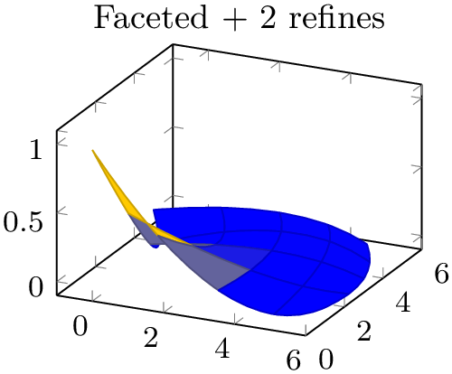
% Preamble: \pgfplotsset{width=7cm,compat=1.18}\usepgfplotslibrary{patchplots}
\foreach \level in {0,1,2} {%
\begin{tikzpicture}
\begin{axis}[
footnotesize,
title={Faceted + \level\ refines},
]
\addplot3 [patch,patch type=biquadratic,shader=faceted,
patch refines=\level,
                              ] coordinates
                  {
(0,0,1) (6,1,0) (5,5,0) (-1,5,0)
(3,1,0) (6,3,0) (2,6,0) (0,3,0)
(3,3.75,0)
};
\end{axis}
\end{tikzpicture}
}
5.9.4Drawing Grids
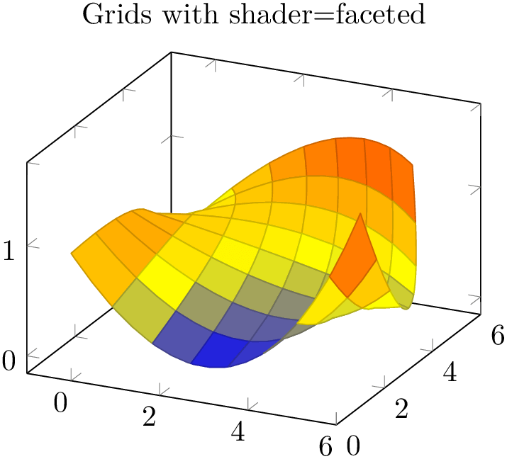
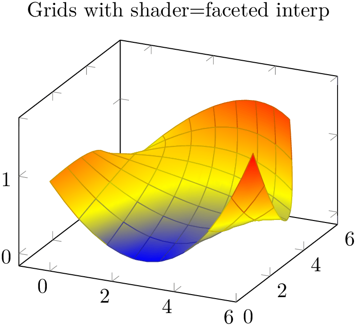
The patchplots library supports grid (mesh) visualization in the same way as for two/three-dimensional mesh and surf plots. This includes four different approaches: the first is shader=faceted, which uses constant fill color and faceted color for stroke paths (as we already saw in Section 5.9.3). The second approach is to use shader=faceted interp which uses interpolated shadings for filling and issues stroke paths on top of each interpolated element. The third approach is to issue two \addplot commands, one with the filled patch plot, and one with a patch,mesh style which only draws (colored) grid lines on top of the previous plot. The three approaches are shown below.
% Preamble: \pgfplotsset{width=7cm,compat=1.18}\usepgfplotslibrary{patchplots}
\begin{tikzpicture}
\begin{axis}[
                      title={Grids with
                  shader=faceted},
]
\addplot3 [patch,patch type=biquadratic,
shader=faceted,patch refines=3,
] coordinates {
(0,0,1) (6,1,1.6) (5,5,1.3) (-1,5,0)
(3,1,0) (6,3,0.4) (2,6,1.1) (0,3,0.9)
(3,3.75,0.5)
};
\end{axis}
\end{tikzpicture}
As already discussed in Section 5.9.3, the approach with shader=faceted works well if the mesh width is small enough (such that single patches do not overlap and their fill area is within the patch boundaries).
% Preamble: \pgfplotsset{width=7cm,compat=1.18}\usepgfplotslibrary{patchplots}
\begin{tikzpicture}
\begin{axis}[
                      title={Grids with shader=faceted
                  interp},
]
\addplot3 [patch,patch type=biquadratic,
                          shader=faceted
                  interp,patch refines=3]
coordinates {
(0,0,1) (6,1,1.6) (5,5,1.3) (-1,5,0)
(3,1,0) (6,3,0.4) (2,6,1.1) (0,3,0.9)
(3,3.75,0.5)
};
\end{axis}
\end{tikzpicture}
Here, grid lines are defined to be the patch boundary, so it may occasionally happen for coarse patches that grid lines cross the filled area. If you experience problems, consider using the patch refines key. The shader=faceted interp supports z buffer – at the cost of generating one shading for each patch element (the stroke path is drawn immediately after the patch element is shaded). This can become quite expensive95 at display time and may lead to huge PDF files. However, shader=faceted interp provides smooth shadings and, at the same time, good grid lines which are drawn in the correct order.
% Preamble: \pgfplotsset{width=7cm,compat=1.18}\usepgfplotslibrary{patchplots}
\begin{tikzpicture}
\begin{axis}[
                      title={Mesh on top of patches
                  (i): obscured},
]
\addplot3 [patch,patch type=biquadratic,
shader=interp,patch refines=3,
] coordinates {
(0,0,1) (6,1,1.6) (5,5,1.3) (-1,5,0)
(3,1,0) (6,3,0.4) (2,6,1.1) (0,3,0.9)
(3,3.75,0.5)
};
\addplot3 [patch,patch type=biquadratic,
mesh,black,patch refines=3,
] coordinates {
(0,0,1) (6,1,1.6) (5,5,1.3) (-1,5,0)
(3,1,0) (6,3,0.4) (2,6,1.1) (0,3,0.9)
(3,3.75,0.5)
};
\end{axis}
\end{tikzpicture}

% Preamble: \pgfplotsset{width=7cm,compat=1.18}\usepgfplotslibrary{patchplots}
\begin{tikzpicture}
\begin{axis}[
                      title={Mesh on top of patches
                  (ii): unobscured\\
\tiny Geometry provided by Prof. Chernov, Bonn},
title style={align=center},
view={156}{28},
]
\addplot3 [patch,patch type=bilinear,
shader=interp,
patch table=plotdata/patchexample_conn.dat,
] file {plotdata/patchexample_verts.dat};
\addplot3 [patch,patch type=bilinear,
mesh,black,
patch table=plotdata/patchexample_conn.dat,
] file {plotdata/patchexample_verts.dat};
\end{axis}
\end{tikzpicture}
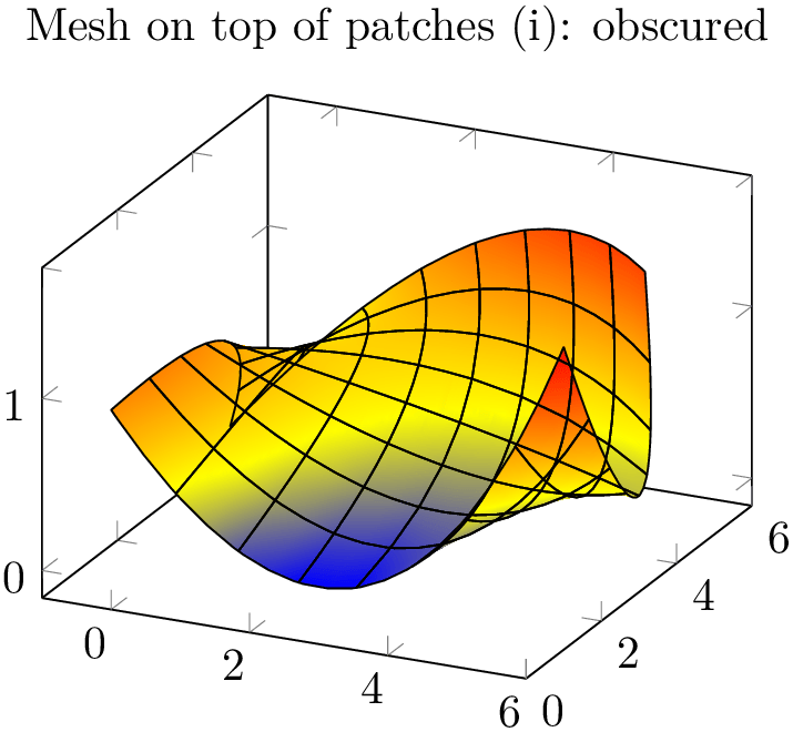
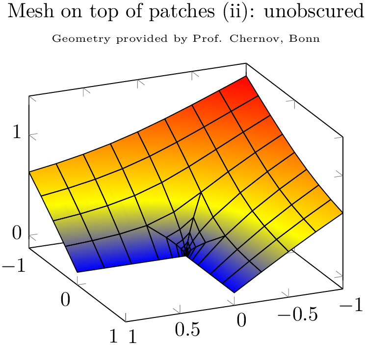
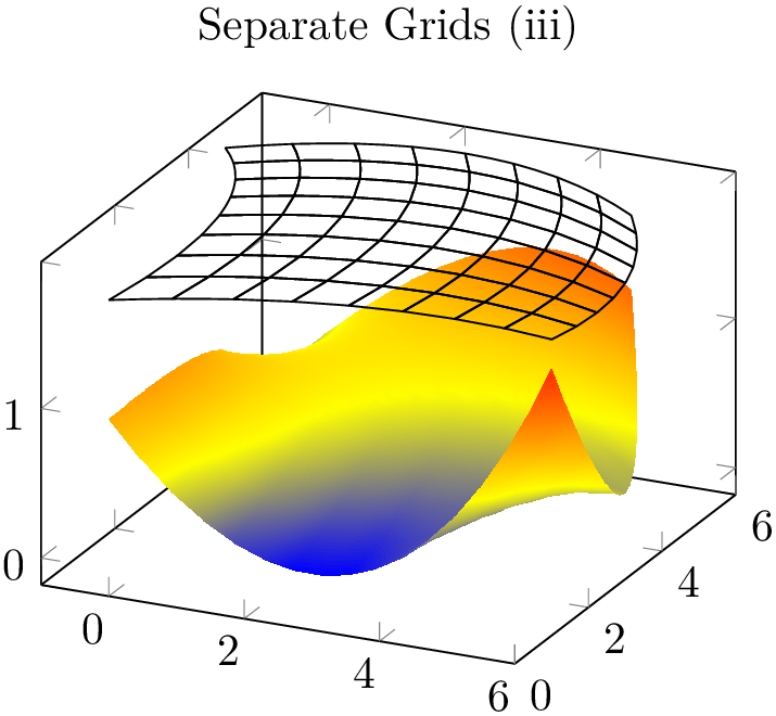
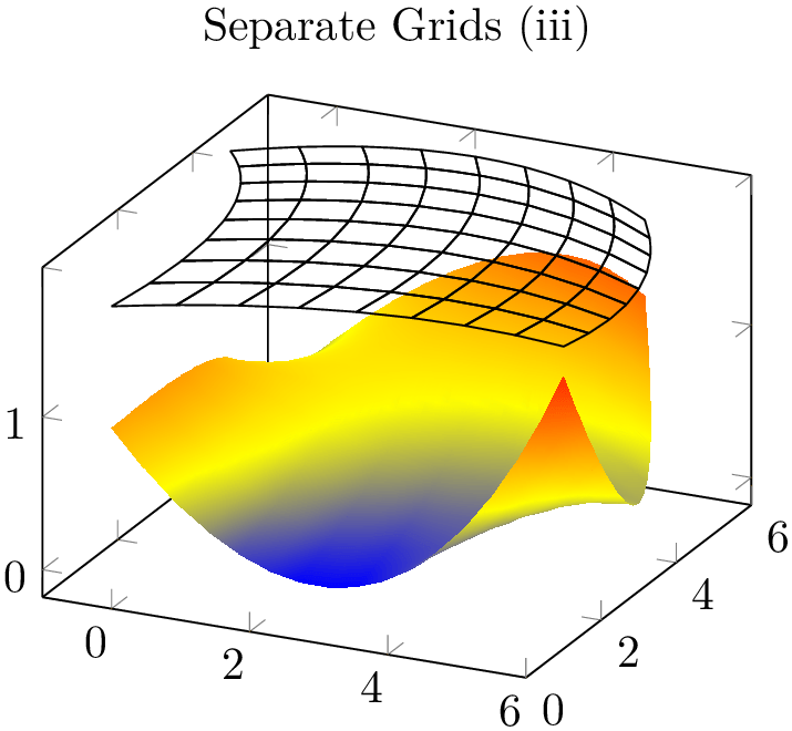
The approach to draw grids separately is done by means of two \addplot statements; the first using patch as before, the second using patch,mesh. This configures pgfplots to visualize just the mesh. Make sure you provide ‘mesh’ after ‘patch’ since the latter activates filled surf visualization. The approach of meshes on top of patches implies to draw grid lines simply over any previous drawing operations. Thus, depth information is lost (as displayed in the first example above). Overlaying grid lines on top of the surface works in special cases (see bottom picture). An approach which always works is to provide the mesh at a fixed \(z\) position as displayed in the following example:
% Preamble: \pgfplotsset{width=7cm,compat=1.18}\usepgfplotslibrary{patchplots}
\begin{tikzpicture}
\begin{axis}[
title={Separate Grids (iii)},
]
\addplot3 [patch,patch type=biquadratic,
shader=interp,patch refines=3,
] coordinates {
(0,0,1) (6,1,1.6) (5,5,1.3) (-1,5,0)
(3,1,0) (6,3,0.4) (2,6,1.1) (0,3,0.9)
(3,3.75,0.5)
};
\addplot3 [patch,patch type=biquadratic,
mesh,black,
z filter/.code={\def\pgfmathresult{1.8}},
patch refines=3,
] coordinates {
(0,0,1) (6,1,1.6) (5,5,1.3) (-1,5,0)
(3,1,0) (6,3,0.4) (2,6,1.1) (0,3,0.9)
(3,3.75,0.5)
};
\end{axis}
\end{tikzpicture}
Here, the first \addplot3 command is the same as above, just with shader=interp. The second reproduces the same geometry, but uses a z filter to fix the \(z\)-coordinate (in this case to \(z=1.8\)). This effectively overrules all \(z\)-coordinates.
Thus, grid lines can be drawn either by means of flat fill color with shader=faceted (efficient), by means of interpolated fill colors with shader=faceted interp (inefficient, see above) or, for special applications, using a separate patch,mesh plot which is drawn on top of the patches (efficient). In any case, the mesh visualization considers the faceted color which can depend on mapped color.