Manual for Package pgfplots
2D/3D Plots in LATeX, Version 1.18.2
https://github.com/pgf-tikz/pgfplots
Related Libraries
5.11Smith Charts
-
\usepgfplotslibrary{smithchart} % LaTeX and plain TeX 
-
\usepgfplotslibrary[smithchart] % ConTeXt 
-
\usetikzlibrary{pgfplots.smithchart} % LaTeX and plain TeX 
-
\usetikzlibrary[pgfplots.smithchart] % ConTeXt 
-
• the data map \(r(z)\) shown above,
-
• an axis class which interprets \(x\) as the real components and \(y\) as the imaginary components,
-
• a visualization of grid lines as arcs,
-
• the possibility to stop grid lines to allow uniform spacing in Smith charts,
-
• a large set of the pgfplots axis fine tuning parameters,
-
• input of already mapped coordinates \(r(z)\) (i.e. Cartesian coordinates in the unit circle),
-
• many of the pgfplots plot handlers.
A library to draw Smith charts.
A Smith chart maps the complex half plane with positive real parts to the unit circle. The smithchart library allows pgfplots to visualize Smith charts: it visualizes two-dimensional input coordinates \(z \in \mathbb {C} \) of the form \(z = x+ j y \in \mathbb {C}\) (\(j\) being the imaginary unit, \(j^2=-1\)) with \(x \ge 0\) using the map \(r\colon [0,\infty ] \times [-\infty ,\infty ]\) \(\to \) \(\{ a+j b \;\vert \; a^2 + b^2 = 1 \}\), \(r(z) = \frac {z-1}{z+1}\) using complex number division. The result is always in the unit circle.
The main application for Smith charts is in the area of electrical and electronics engineers specializing in radio frequency: to show the reflection coefficient \(r(z)\) for normalised impedance \(z\). It is beyond the scope of this manual to delve into the radio frequency techniques; for us, it is important to note that the smithchart library supports
5.11.1Smith Chart Axes
-
\begin{smithchart}[
 options
 ]
]
-
 environment contents
-
\end{smithchart}
-
/pgfplots/smithchart mirrored=true|false (initially false) 
The \begin{smithchart} environment draws Smith charts. It accepts
the same
 options
 as \begin{axis}. In fact, it is equivalent to
\begin{axis}[
 options
 ,axis type=smithchart].
% Preamble: \pgfplotsset{width=7cm,compat=1.18}\usepgfplotslibrary{smithchart}
\begin{tikzpicture}
\begin{smithchart}[
title=Impedance Smith Chart,
]
                        \addplot coordinates
                    {
(0.5,0.2) (1,0.8) (2,2)
};
\end{smithchart}
\end{tikzpicture}
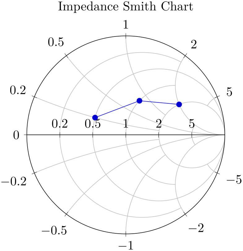
The example above visualizes three data points using the initial configuration of Smith charts; the data points are interpreted as complex numbers \(z = x + j y\) and are mapped using \(r(z)\).
Here, the \(x\)-coordinate refers to the cycles described by the horizontal line whereas the \(y\)-coordinate refers to the cycles described by the tick labels on the outside.
This key is deprecated. Its output does not resemble Admittance Smith charts because the author failed to understand how to render them completely.
pgfplots currently supports no Admittance Smith charts. Contributors are free to submit patches which correct the behavior.
Existing code relying on smithchart mirrored still produces the same as before, but the code generates a warning.
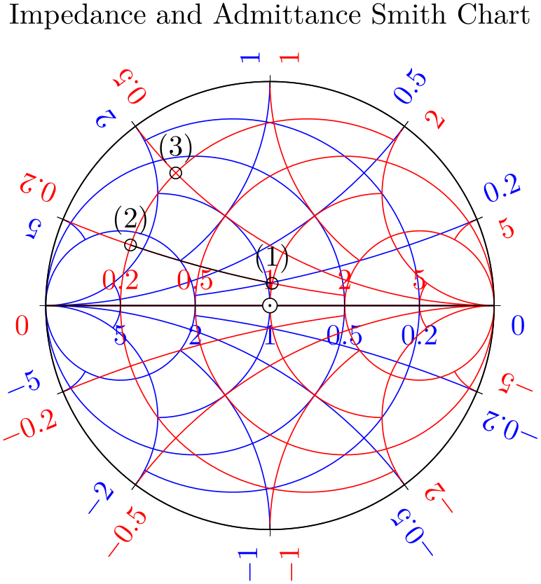
Since pgfplots can draw two axes on top of each other, a combined Impedance/Admittance Smith chart is also possible.
% Preamble: \pgfplotsset{width=7cm,compat=1.18}\usepgfplotslibrary{smithchart}
\begin{tikzpicture}[]
% First, the Admittance chart:
\begin{smithchart}[
title=Impedance and Admittance Smith Chart,
smithchart mirrored,
xticklabel shift=-19pt,
grid style={blue},
ticklabel style={blue},
yticklabel around circle,
]
\end{smithchart}
% Second, overlay the impedance chart:
\begin{smithchart}[
show origin,
grid style={red},
ticklabel style={red},
yticklabel around circle*,
]
                            \addplot+
                    [black,mark=o,only marks,point meta=explicit symbolic,nodes near coords]
                                coordinates
                    {
(0.2,0.2) [(2)]
(1,0.2) [(1)]
};
                            \addplot+
                    [black,no markers,domain=0.2:1] {0.2};
                            \addplot+
                    [black,mark=o,only marks,point meta=explicit symbolic,nodes near coords]
coordinates{
(0.2,0.5) [(3)]
};
\end{smithchart}
\end{tikzpicture}
Since such a chart easily becomes crowded, it should be tuned manually by means of “suitable” appearance options (if you feel that there is a “suitable default”, let me know).
Details for show origin, yticklabel around circle, and yticklabel around circle* can be found later in this section.
5.11.2Size Control
A Smith chart can be resized by providing either width or height as argument to the axis. If you provide both, the Chart is drawn as an ellipsis.
The tick and grid positions for smithchart axes are realized by means of three manually tuned sets of grid lines: one for small-sized plots, one for medium-sized plots and one for huge plots. The actual parameters for width or height are considered to select one of the following sets:
-
/pgfplots/few smithchart ticks(style, no value) 
-
• copy–paste the definition above and adjust it or
-
• omit all the default smithchart xtick/.style stuff and write xtick={
 your list
 } directly.
This produces the output of the example above – it constitutes the initial configuration for Smith chart which has a width of less than 14cm.
The few smithchart ticks style is defined by:
\pgfplotsset{
few smithchart ticks/.style={
default smithchart xtick/.style={
xtick={0.2,0.5,1,2,5},
},
default smithchart ytick/.style={
ytick={%
0,%
0.2, 0.5, 1, 2, 5,%
-0.2,-0.5,-1,-2,-5},
},
default smithchart xytick/.style={
xgrid each nth passes y={2},
ygrid each nth passes x={2},
},
},
}
Note that few smithchart ticks contains syntactical overhead to distinguish between “default ticks” and final tick positions: it does not assign xtick and ytick directly. Instead, it provides them as separate default xtick style arguments. The purpose of this distinction is to mark them as “default” arguments – the underlying styles smithchart/every default xtick is used if and only if there is no xtick value given.
In case you want to override this default, you can either
As mentioned, the only purpose of the
default smithchart xtick/.style
overhead is to distinguish between \begin{smithchart}[xtick={ user defined
 }] and default arguments (see the documentation of
default smithchart xtick/.style
for more about this technical detail).
For fine tuning of the scaling decisions, see the smith chart ticks by size key.
-
/pgfplots/many smithchart ticks(style, no value) 
The many smithchart ticks style is used for every Smith chart whose width exceeds 14cm although it is less than 20cm:
% Preamble: \pgfplotsset{width=7cm,compat=1.18}\usepgfplotslibrary{smithchart}
\begin{tikzpicture}
\begin{smithchart}[
title=Medium-Sized Smith Chart,
width=14cm,
]
\addplot coordinates {(0.5,0.2) (1,0.8) (2,2)};
\end{smithchart}
\end{tikzpicture}
We see that many smithchart ticks has different placement and alignment options than few smithchart ticks: it uses sloped tick labels inside of the unit circle for the \(y\) descriptions (imaginary axis).
The initial configuration is realized by means of two separate styles: one which defines only the tick positions (the many smithchart ticks* style) and one which also changes placement and alignment options. The initial configuration can be changed individually (see the end of this section for examples). The initial configuration is:
\pgfplotsset{
many smithchart ticks*/.style={
default smithchart xtick/.style={
xtick={
0.1,0.2,0.3,0.4,0.5,1,1.5,2,3,4,5,10,20%
},
minor xtick={0.6,0.7,0.8,0.9,1.1,1.2,1.3,1.4,1.6,1.7,1.8,1.9,
2.2,2.4,2.6,2.8,3.2,3.4,3.6,3.8,4.5,6,7,8,9,50},
},
default smithchart ytick/.style={
ytick={%
0,%
0.1,0.2,...,1,1.5,2,3,4,5,10,20,%
-0.1,-0.2,...,-1,-1.5,-2,-3,-4,-5,-10,-20%
},
minor ytick={%
1.1,1.2,1.3,1.4,1.6,1.7,1.8,1.9,2.2,2.4,2.6,2.8,3.2,3.4,3.6,3.8,
4.5,6,7,8,9,50,%
-1.1,-1.2,-1.3,-1.4,-1.6,-1.7,-1.8,-1.9,-2.2,-2.4,-2.6,-2.8,
-3.2,-3.4,-3.6,-3.8,-4.5,-6,-7,-8,-9,-50%
},
},
default smithchart xytick/.style={
xgrid each nth passes y={1,2,4,5,10,20},
ygrid each nth passes x={1,2,3,5,10:3,20:3},
},
},
/pgfplots/many smithchart ticks/.style={
many smithchart ticks*,
yticklabel in circle,
show origin=true,
},
}
See the documentation for few smithchart ticks for an explanation of the default smithchart xtick/.style overhead.
-
/pgfplots/dense smithchart ticks(style, no value) 
The dense smithchart ticks style assigns the set of tick positions for every Smith chart whose width is at least 20cm:
% Preamble: \pgfplotsset{width=7cm,compat=1.18}\usepgfplotslibrary{smithchart}
\begin{tikzpicture}[scale=0.75]
\begin{smithchart}[
title=Huge Smith Chart (rescaled),
width=20cm,
]
\addplot coordinates {(0.5,0.2) (1,0.8) (2,2)};
\end{smithchart}
\end{tikzpicture}
Attention: This style might change in future versions!
Similarly to many smithchart ticks (see above), the initial configuration is realized by means of two separate styles: one which defines only the tick positions (the many smithchart ticks* style) and one which also changes placement and alignment options:
\pgfplotsset{
dense smithchart ticks*/.style={
default smithchart xtick/.style={
xtick={
0.1,0.2,0.3,0.4,0.5,0.6,0.7,0.8,0.9,1,1.2,1.4,1.6,1.8,2,3,4,5,10,20%
},
minor xtick={%
0.01,0.02,0.03,0.04,0.05,0.06,0.07,0.08,0.09,0.11,0.12,0.13,0.14,0.15,0.16,0.17,
0.18,0.19,0.22,0.24,0.26,0.28,0.32,0.34,0.36,0.38,0.42,0.44,0.46,0.48,%
                                    0.52,%
                    This is sub-optimal and will (hopefully) be improved in the future.
0.55,0.65,0.75,0.85,0.95,%
                                    %
                    0.6,0.7,0.8,0.9,%
1.1,1.3,1.5,1.7,1.9,%
2.2,2.4,2.6,2.8,3.2,3.4,3.6,3.8,4.5,6,7,8,9,50},
},
default smithchart ytick/.style={
ytick={%
0,%
0.1,0.2,...,1,1.2,1.4,1.6,1.8,2,3,4,5,10,20,%
-0.1,-0.2,...,-1,-1.2,-1.4,-1.6,-1.8,-2,-3,-4,-5,-10,-20%
},
minor ytick={%
0.01,0.02,0.03,0.04,0.05,0.06,0.07,0.08,0.09,0.11,0.12,0.13,0.14,0.15,0.16,0.17,
0.18,0.19,0.22,0.24,0.26,0.28,0.32,0.34,0.36,0.38,0.42,0.44,0.46,0.48,%
0.55,0.65,0.75,0.85,0.95,%
1.1,1.3,1.5,1.7,1.9,2.2,2.4,2.6,2.8,3.2,3.4,3.6,3.8,4.5,6,7,8,9,50,%
-0.01,-0.02,-0.03,-0.04,-0.05,-0.06,-0.07,-0.08,-0.09,-0.11,-0.12,-0.13,-0.14,
-0.15,-0.16,-0.17,-0.18,-0.19,-0.22,-0.24,-0.26,-0.28,-0.32,-0.34,-0.36,-0.38,
-0.42,-0.44,-0.46,-0.48,-0.55,-0.65,-0.75,-0.85,-0.95,%
-1.1,-1.3,-1.5,-1.7,-1.9,-2.2,-2.4,-2.6,-2.8,-3.2,-3.4,-3.6,-3.8,-4.5,-6,-7,-8,
-9,-50%
},
},
default smithchart xytick/.style={
xgrid each nth passes y={0.2 if < 0.2001,0.5 if < 0.50001,1 if < 1.001,2,4,5,10,20},
ygrid each nth passes x={0.2 if < 0.2001,0.52 if < 0.52001,1 if < 1.001,2,3,5,10:3,20:3},
},
},
dense smithchart ticks/.style={
yticklabel in circle,
dense smithchart ticks*,
show origin=true,
every major grid/.style={black!60},
},
}
See the documentation for few smithchart ticks for an explanation of the default smithchart xtick/.style overhead.
-
/pgfplots/default smithchart xtick(no value) 
-
/pgfplots/default smithchart ytick(no value) 
-
/pgfplots/default smithchart xytick(no value) 
The default smithchart xtick style is installed if and only if you do not provide xtick manually.
Similarly, the default smithchart ytick style is installed if and only if you do not provide ytick manually.
Finally, the default smithchart xytick style is installed if and only if you provide neither xtick nor ytick.
These styles are usually defined in few smithchart ticks and its variants, see above.
5.11.3Working with Prepared Data
-
/pgfplots/is smithchart cs=true|false (initially false) 
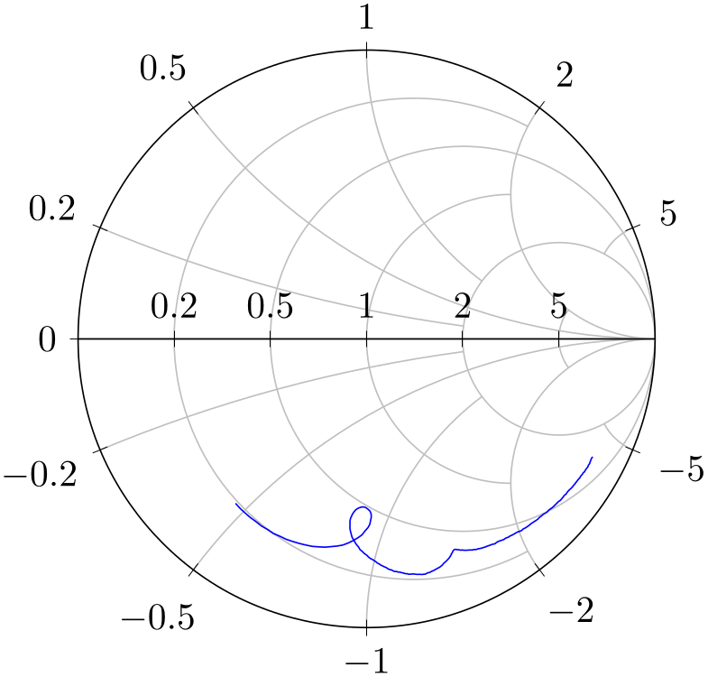
Occasionally, you may already have input data transformed into unit circle Cartesian coordinate \(r(z) = (x,y)\).
You can provide them to pgfplots with the is smithchart cs key:

% Preamble: \pgfplotsset{width=7cm,compat=1.18}\usepgfplotslibrary{smithchart}
\begin{tikzpicture}
\begin{smithchart}
% smithchart_data.dat contains
% 0.78395 -0.40845
% 0.78165 -0.41147
% 0.77934 -0.41466
% 0.77774 -0.41869
% ...
\addplot [
blue,
is smithchart cs,
] file {plotdata/smithchart_data.dat};
\end{smithchart}
\end{tikzpicture}
Using is smithchart cs tells pgfplots to skip the transformation \(r(z)\).
5.11.4Appearance Control and Styles
-
/pgfplots/show origin=true|false (initially false) 
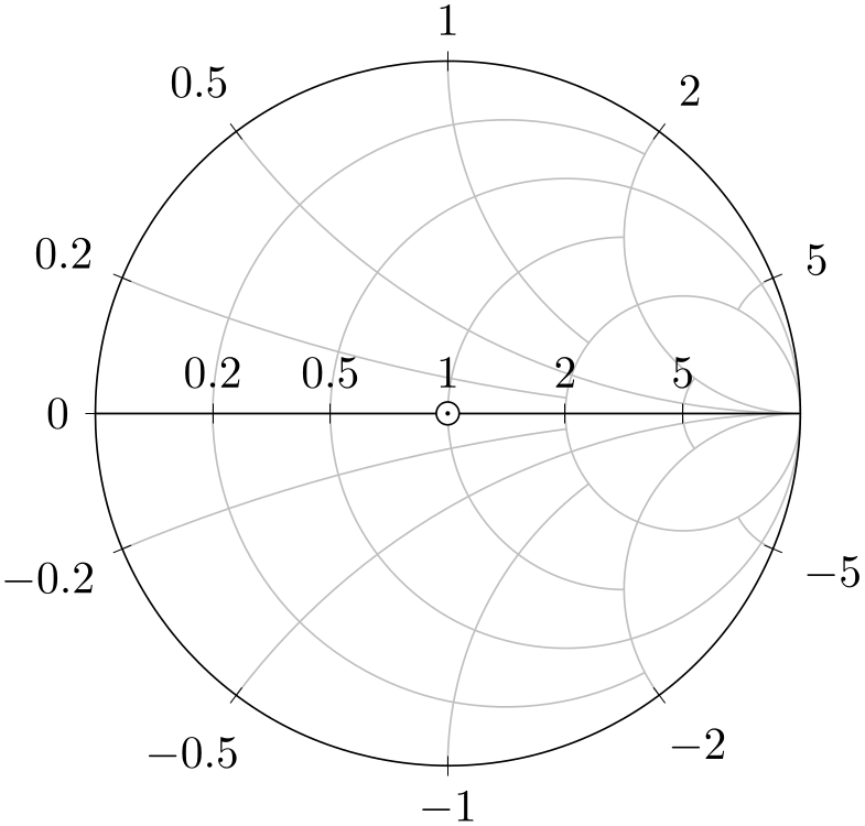
Allows to place an extra description at the point \((0,0)\) to mark the origin.

% Preamble: \pgfplotsset{width=7cm,compat=1.18}\usepgfplotslibrary{smithchart}
\begin{tikzpicture}
\begin{smithchart}[
show origin,
]
\end{smithchart}
\end{tikzpicture}
-
/pgfplots/yticklabel in circle(style, no value) 
This style draws Smith chart tick labels for imaginary components (the ytick arguments) inside of the circle.
It installs transformations to rotate and shift tick labels. See the many smithchart ticks style for an example.
The initial configuration for this style is
\pgfplotsset{
yticklabel in circle/.style={
ytick align=inside,
yticklabel style={
rotate=90,
sloped like y axis={
                                    execute
                    for upside down={\tikzset{anchor=north east}},
                                    % allow
                    upside down,
                                    reset
                    nontranslations=false},
anchor=south west,
% font=\tiny,
},
},
}
-
/pgfplots/yticklabel around circle(style, no value) 
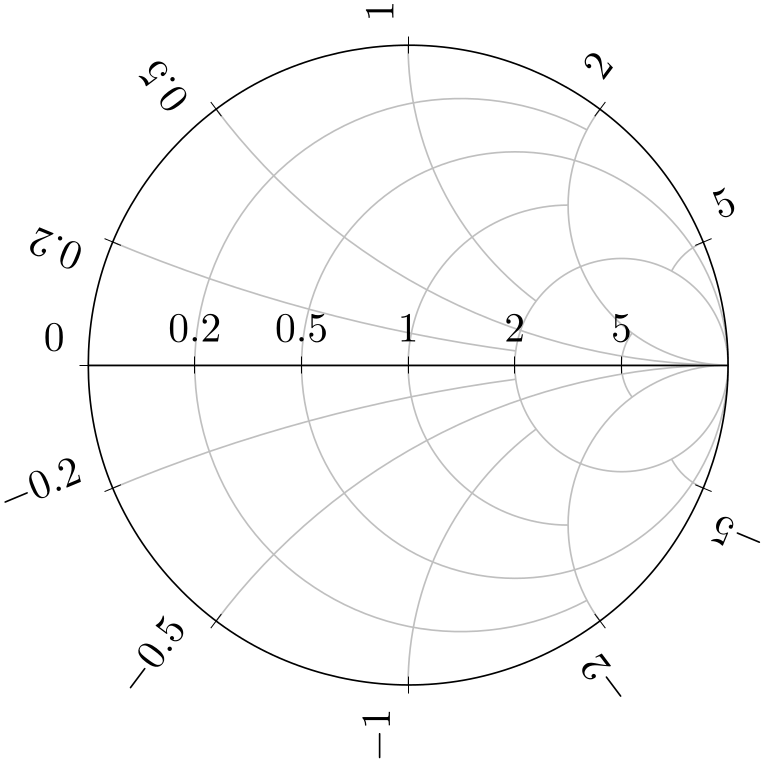
This style draws Smith chart tick labels for imaginary components (the ytick arguments) outside of the circle, but rotated to fit the slope of the circle.
% Preamble: \pgfplotsset{width=7cm,compat=1.18}\usepgfplotslibrary{smithchart}
\begin{tikzpicture}
\begin{smithchart}[
yticklabel around circle,
]
\end{smithchart}
\end{tikzpicture}
The initial configuration for this style is
\pgfplotsset{
yticklabel around circle/.style={
ytick align=center,
yticklabel style={
rotate=90,
sloped like y axis={
                                    execute
                    for upside down={\tikzset{anchor=south west}},
                                    % allow
                    upside down,
                                    reset
                    nontranslations=false},
anchor=south east,
},
},
}
-
/pgfplots/yticklabel around circle*(style, no value) 
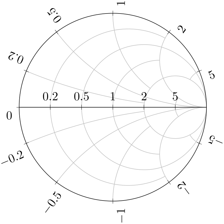
A variant of yticklabel around circle which exchanges the anchors:
% Preamble: \pgfplotsset{width=7cm,compat=1.18}\usepgfplotslibrary{smithchart}
\begin{tikzpicture}
\begin{smithchart}[
yticklabel around circle*,
]
\end{smithchart}
\end{tikzpicture}
If you have two Smith charts in the same figure, you can overlay them if the first uses yticklabel around circle and the second uses yticklabel around circle* (see the beginning of this section for an example).
The initial configuration for this style is
\pgfplotsset{
yticklabel around circle*/.style={
ytick align=center,
yticklabel style={
rotate=90,
sloped like y axis={
                                    execute
                    for upside down={\tikzset{anchor=north west}},
                                    % allow
                    upside down,
                                    reset
                    nontranslations=false},
anchor=north east,
},
},
}
-
/pgfplots/every smithchart axis(style, no value) 
This style is installed for every Smith chart. It is defined as
\pgfplotsset{
every smithchart axis/.style={
grid=both,
xmin=0,
scaled ticks=false, % never draw the \cdot 10^4 labels
major tick style={draw=black},
xtick align=center,
ytick align=center,
},
}
5.11.5Controlling Arcs and Their Stop Points
This section allows advanced control over Smith chart arcs (grid lines). The two features xgrid each nth passes y and xgrid stop at y (and their counterparts for \(y\)) allow to draw only partial arcs in order to get a more uniform appearance.
-
/pgfplots/xgrid each nth passes y={
 list of stop entries
 } (initially empty)
-
1. single \(y\)-coordinates, for example xgrid each nth passes y={1,2} or
-
2. the same as above, followed by an integer, for example xgrid each nth passes y={1:3,2:2} or
-
3. an additional restriction clause like xgrid each nth passes y={0.2 if <0.3}.
In this case, the all \(x\) grid lines which fulfill \(x \le 0.3\) will be checked if they are allowed to pass \(y=0.2\). All \(x\) grid lines with \(x > 0.3\) are not affected by the constraint. See the dense smithchart ticks style for an application example.
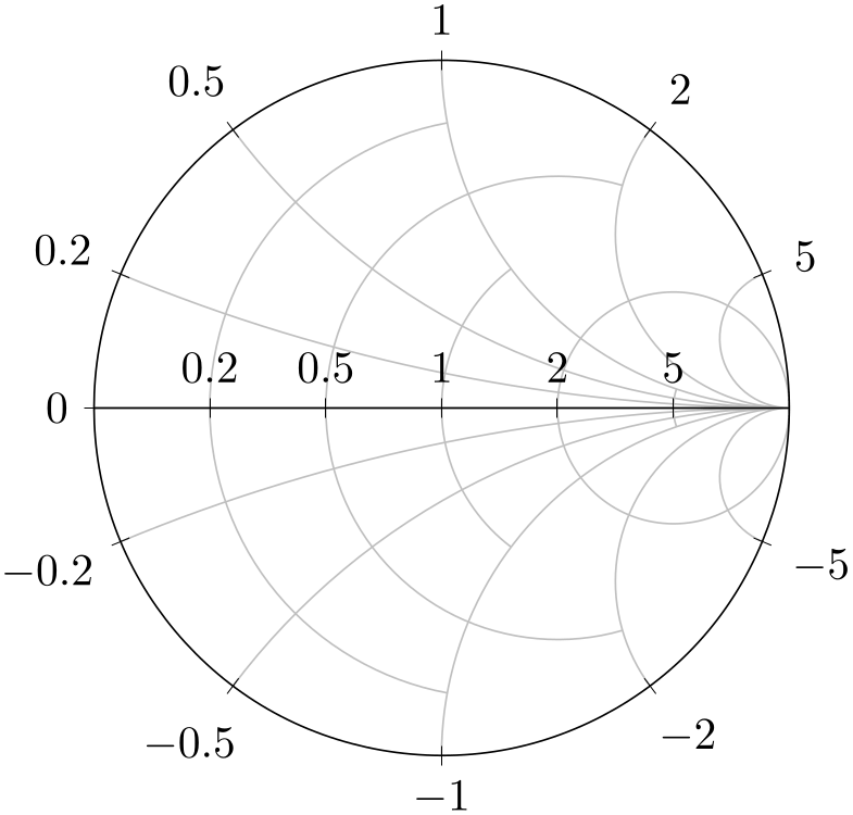
This key constitutes the main idea to draw only partial arcs: you provide a couple of \(y\) tick coordinates which constitute “boundaries”. Then, only each (say) second \(x\) grid line is allowed to pass these boundaries:
% Preamble: \pgfplotsset{width=7cm,compat=1.18}\usepgfplotslibrary{smithchart}
\begin{tikzpicture}
\begin{smithchart}[
xtick={0.2,0.5,1,2,5},
ytick={
0,
0.2, 0.5, 1, 2, 5,
-0.2,-0.5,-1,-2,-5
},
xgrid each nth passes y={1,2},
]
\end{smithchart}
\end{tikzpicture}
The example overwrites the default smithchart ticks to define a new layout: now, every ytick uses the complete arc, but some of the grid lines for xtick stop at \(y=1\) and, if they pass, they may stop at \(y=2\).
The argument
 list of stop entries
 is a comma-separated list of entries. Each entry is, in the simplest case, a \(y\)-coordinate (it should be a coordinate
which appears in the ytick list). This simplest case
means “only each second \(x\) grid line may pass the grid line for this \(y\)”. The second syntax allows to
provide a natural number, using
 y coord
 :
: number
 . This means to let only each
 number
 ’s \(x\) grid line pass the designated \(y\) grid line. The third syntax also allows to write if <
  x value
 . It means the entry is considered only for \(x\) grid lines which are less than
 x value
 . To summarize: there are the three possible forms of entries
Note that xgrid each nth passes y always employs symmetry; you do not need to provide \(y\) and \(-y\) (if you want to, you may use the xgrid stop at y key to overrule the “each nth” strategy).
In order to check if a given xtick argument is the “\(n\)th” grid line, pgfplots collects all xtick and minor xtick arguments into one large array and sorts it. Then, it uses the resulting sequence to assign the indices. Consequently, you can freely intermix minor and major ticks; it will still work. The only way to affect the counting is the xgrid each nth passes y start key, see below.
-
/pgfplots/ygrid each nth passes x={
 list of stop entries
 } (initially empty)
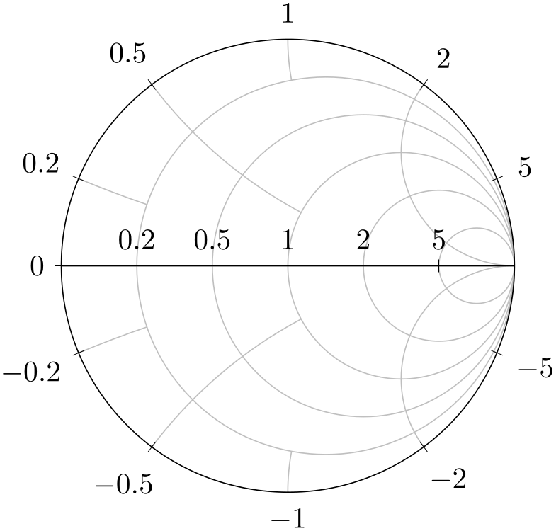
As you may already have guessed, this is the \(y\) counterpart of xgrid each nth passes y. It restricts the arcs for \(y\) grid lines by provided \(x\) ticks:
% Preamble: \pgfplotsset{width=7cm,compat=1.18}\usepgfplotslibrary{smithchart}
\begin{tikzpicture}
\begin{smithchart}[
xtick={0.2,0.5,1,2,5},
ytick={
0,
0.2, 0.5, 1, 2, 5,
-0.2,-0.5,-1,-2,-5
},
ygrid each nth passes x={0.2,1:2},
]
\end{smithchart}
\end{tikzpicture}
The syntax is exactly the same as explained for xgrid each nth passes y. The only difference is that the if < syntax uses absolute values \(|y|\) (to maintain symmetry).
Now, we know how to use xgrid each nth passes y and the corresponding ygrid each nth passes x separately. Can we use both keys at the same time? Yes – but it may happen that lines end in white space! pgfplots applies some logic to avoid arcs ending in white space by extending them to the next feasible stopping point. The result of mixing both of these keys is thus corrected automatically.
-
/pgfplots/xgrid each nth passes y start={
 integer
 } (initially 0)
-
/pgfplots/ygrid each nth passes x start={
 integer
 } (initially 0)
Allows to modify where the “each \(n\)th” counting starts. The argument can be considered as a shift. I consider this key to be more or less experimental – in the hope it may be useful. Try it out.
-
/pgfplots/xgrid stop at y={
 list
list } (initially empty)
-
/pgfplots/ygrid stop at x={
 list
list } (initially empty)
These keys allow to provide individual stop points for explicitly chosen tick positions. These explicit stop points have higher precedence over the each nth features described above.
The ygrid stop at x key accepts a comma-separated
list of entries
 y coord
 :
: x stop point
 :
:
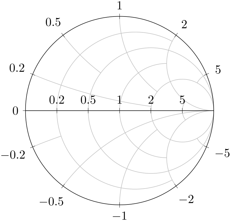
% Preamble: \pgfplotsset{width=7cm,compat=1.18}\usepgfplotslibrary{smithchart}
\begin{tikzpicture}
\begin{smithchart}[
ygrid stop at x={0.5:0.5,-0.2:0.2}
]
\end{smithchart}
\end{tikzpicture}
In this example, the \(y=0.5\) arc stops at the \(x=0.5\) arc whereas the \(y=-0.2\) arc stops at \(x=0.2\).
The ygrid stop at x key allows asymmetric layouts (different stop points for \(y\) and \(-y\)).

