pgfplots

Related Libraries

\(\newcommand{\footnotename}{footnote}\) \(\def \LWRfootnote {1}\) \(\newcommand {\footnote }[2][\LWRfootnote ]{{}^{\mathrm {#1}}}\) \(\newcommand {\footnotemark }[1][\LWRfootnote ]{{}^{\mathrm {#1}}}\) \(\let \LWRorighspace \hspace \) \(\renewcommand {\hspace }{\ifstar \LWRorighspace \LWRorighspace }\) \(\newcommand {\mathnormal }[1]{{#1}}\) \(\newcommand \ensuremath [1]{#1}\) \(\newcommand {\LWRframebox }[2][]{\fbox {#2}} \newcommand {\framebox }[1][]{\LWRframebox } \) \(\newcommand {\setlength }[2]{}\) \(\newcommand {\addtolength }[2]{}\) \(\newcommand {\setcounter }[2]{}\) \(\newcommand {\addtocounter }[2]{}\) \(\newcommand {\arabic }[1]{}\) \(\newcommand {\number }[1]{}\) \(\newcommand {\noalign }[1]{\text {#1}\notag \\}\) \(\newcommand {\cline }[1]{}\) \(\newcommand {\directlua }[1]{\text {(directlua)}}\) \(\newcommand {\luatexdirectlua }[1]{\text {(directlua)}}\) \(\newcommand {\protect }{}\) \(\def \LWRabsorbnumber #1 {}\) \(\def \LWRabsorbquotenumber "#1 {}\) \(\newcommand {\LWRabsorboption }[1][]{}\) \(\newcommand {\LWRabsorbtwooptions }[1][]{\LWRabsorboption }\) \(\def \mathchar {\ifnextchar "\LWRabsorbquotenumber \LWRabsorbnumber }\) \(\def \mathcode #1={\mathchar }\) \(\let \delcode \mathcode \) \(\let \delimiter \mathchar \) \(\def \oe {\unicode {x0153}}\) \(\def \OE {\unicode {x0152}}\) \(\def \ae {\unicode {x00E6}}\) \(\def \AE {\unicode {x00C6}}\) \(\def \aa {\unicode {x00E5}}\) \(\def \AA {\unicode {x00C5}}\) \(\def \o {\unicode {x00F8}}\) \(\def \O {\unicode {x00D8}}\) \(\def \l {\unicode {x0142}}\) \(\def \L {\unicode {x0141}}\) \(\def \ss {\unicode {x00DF}}\) \(\def \SS {\unicode {x1E9E}}\) \(\def \dag {\unicode {x2020}}\) \(\def \ddag {\unicode {x2021}}\) \(\def \P {\unicode {x00B6}}\) \(\def \copyright {\unicode {x00A9}}\) \(\def \pounds {\unicode {x00A3}}\) \(\let \LWRref \ref \) \(\renewcommand {\ref }{\ifstar \LWRref \LWRref }\) \( \newcommand {\multicolumn }[3]{#3}\) \(\require {textcomp}\) \( \newcommand {\meta }[1]{\langle \textit {#1}\rangle } \) \(\newcommand {\toprule }[1][]{\hline }\) \(\let \midrule \toprule \) \(\let \bottomrule \toprule \) \(\def \LWRbooktabscmidruleparen (#1)#2{}\) \(\newcommand {\LWRbooktabscmidrulenoparen }[1]{}\) \(\newcommand {\cmidrule }[1][]{\ifnextchar (\LWRbooktabscmidruleparen \LWRbooktabscmidrulenoparen }\) \(\newcommand {\morecmidrules }{}\) \(\newcommand {\specialrule }[3]{\hline }\) \(\newcommand {\addlinespace }[1][]{}\) \(\require {colortbl}\) \(\let \LWRorigcolumncolor \columncolor \) \(\renewcommand {\columncolor }[2][named]{\LWRorigcolumncolor [#1]{#2}\LWRabsorbtwooptions }\) \(\let \LWRorigrowcolor \rowcolor \) \(\renewcommand {\rowcolor }[2][named]{\LWRorigrowcolor [#1]{#2}\LWRabsorbtwooptions }\) \(\let \LWRorigcellcolor \cellcolor \) \(\renewcommand {\cellcolor }[2][named]{\LWRorigcellcolor [#1]{#2}\LWRabsorbtwooptions }\) \(\newcommand {\intertext }[1]{\text {#1}\notag \\}\) \(\let \Hat \hat \) \(\let \Check \check \) \(\let \Tilde \tilde \) \(\let \Acute \acute \) \(\let \Grave \grave \) \(\let \Dot \dot \) \(\let \Ddot \ddot \) \(\let \Breve \breve \) \(\let \Bar \bar \) \(\let \Vec \vec \) \(\newcommand {\nicefrac }[3][]{\mathinner {{}^{#2}\!/\!_{#3}}}\)

5.1Clickable Plots

\usepgfplotslibrary{clickable} % LaTeX and plain TeX ¶

\usepgfplotslibrary[clickable] % ConTeXt ¶

\usetikzlibrary{pgfplots.clickable} % LaTeX and plain TeX ¶

\usetikzlibrary[pgfplots.clickable] % ConTeXt ¶

A library which generates small popups whenever one clicks into a plot. The popup displays the coordinate under the mouse pointer, supporting the optional “snap to nearest” clickable coords feature with customizable displayed information. Furthermore, the library allows to display slopes if one holds the mouse pressed and drags it to another point in the plot.

The library has two purposes: to compute slopes in a simple way⁸⁰ and to provide related, optional information to single data points which are not important enough to be listed in the main text (like prototype parameters or other technical things).

⁸⁰ The author is applied mathematician…

5.1.1Overview¶

It is completely sufficient to write


\usepgfplotslibrary{clickable}

in the document preamble. This will automatically prepare every plot.

The library works with Acrobat JavaScript and pdf forms: every plot becomes a push button.

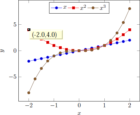
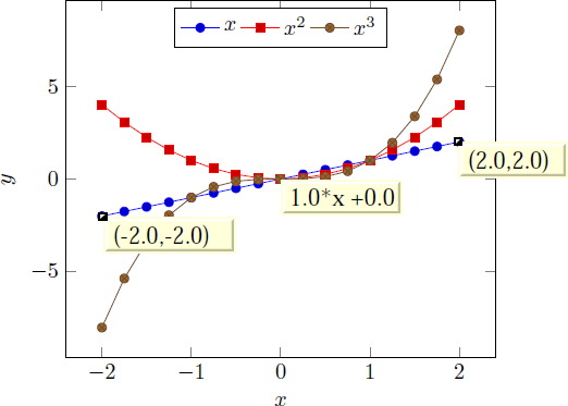
These screenshots show the result of clicking into the axis range (left column) and of dragging from one point to another (right column). The second case shows the result of Drag-and-Drop: it displays start and end points and the equation for the line segment between between the first point of the drag and drop and the second point where the mouse has been released. The line segment is

\[ l(x; x_0,y_0,x_1,y_1) = m \cdot x + n \]

where \(m = (y_1-y_0) / (x_1-x_0)\) is the slope and \(n\) the offset chosen such that \(l(x_0;\dotsc ) = y_0\). For logarithmic plots, logarithms will be applied before computing slopes.

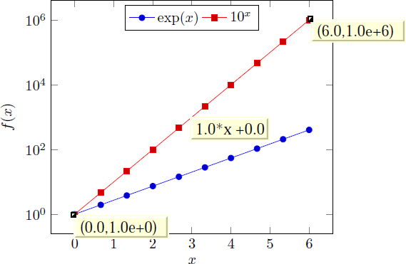
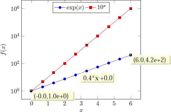
These screen shots show the result of drag- and drop for logarithmic axes: the end points show, again, the coordinates (without logs) and the form field in the middle shows the slope and offset of the linear equation in log coordinates.

The log basis for any logarithmic axes is usually \(10\), but it respects the current setting of log basis x and log basis y. The applied log will always use the same logarithm which is also used for the axis descriptions (this is not necessarily the same as used by PgfplotsTable!).

This document has been produced with the clickable library, so it is possible to load it into Acrobat Reader and simply click into a plot.

/pgfplots/clickable coords={ (math image) displayed text} ¶

Activates a “snap to nearest” feature when clicking onto plot coordinates. The (math image) displayed text is the coordinate’s \(x\) and \(y\) value by default (i.e. you write just clickable coords without an equal sign).


\begin{tikzpicture}


\begin{loglogaxis}[


    clickable coords={


        Level \thisrow{level} (q=\thisrow{q})

},


    \addplot table [x=dof,y=error] {


        level  dof      error           q


        1      4        2.50000000e-01  48


        2      16       6.25000000e-02  25


        3      64       1.56250000e-02  41


        4      256      3.90625000e-03  8


        5      1024     9.76562500e-04  22


        6      4096     2.44140625e-04  46


        7      16384    6.10351562e-05  40


        8      65536    1.52587891e-05  3


        9      262144   3.81469727e-06  1


        10     1048576  9.53674316e-07  9

};


\end{loglogaxis}


\end{tikzpicture}

Now, clicking onto a data point yields ‘Level 7 (q=40)’ whereas clicking besides a data point results in the click coordinates as before,

(math image) displayed text. As an example, we consider again the scatter/classes example of Section 4.5.12:


\begin{tikzpicture}


\begin{axis}[


    clickable coords={(xy): \thisrow{label}},


    scatter/classes={


        a={mark=square*,blue},


        b={mark=triangle*,red},


        c={mark=o,draw=black}   % <-- don't add comma


    \addplot [


        only marks,


        scatter,


        scatter src=explicit symbolic


    ] table [meta=label] {


        x     y      label


        0.1   0.15   a


        0.45  0.27   c


        0.02  0.17   a


        0.06  0.1    a


        0.9   0.5    b


        0.5   0.3    c


        0.85  0.52   b


        0.12  0.05   a


        0.73  0.45   b


        0.53  0.25   c


        0.76  0.5    b


        0.55  0.32   c

};


\end{axis}


\end{tikzpicture}

Here, we find popups like

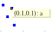
(math image) displayed text is a richtext string displayed with JavaScript. For most purposes, it is used like an unformatted C string: it contains characters, perhaps line breaks with ‘\n’ or tabulators with ‘\t’, but it should not contain TeX formatting instructions, especially no math mode (the ‘(xy)’ replacement text is formatted with sprintf, see below). Consider clickable coords code in case you’d like to preprocess data before displaying it. If you experience problems with special characters, try prepending a backslash to them. If that doesn’t work either, try to prefix the word with ‘\\’ and/or with ‘\string’. Consider using clickable coords size if you intend to work with multiline fields and the size allocation needs improvements.

In fact, (math image) displayed text can even contain richtext (=XHTML) formatting instructions like ‘’ (note the final slash) or ‘text’ (note the backslash before ‘#’) which changes the color for text. The arguments are CSS fields, consider an HTML reference for a list of CSS attributes.

It is possible to use clickable coords together with three dimensional axes. Note that dynamic (clickable) features of a three dimensional axis without clickable coords will be disabled (they appear to be useless). Furthermore, three dimensional axes do not support slope calculations; only the “snap to nearest” feature is available.

Consider using annot/snap dist=6 to increase the “snap to nearest” distance.

The clickable coords can be specified for all plots in an axis (as in the examples above), but also once for every single \addplot commands for which the “snap to nearest” feature is desired (with different (math image) displayed text).

If multiple clickable coords are on the same position, each click chooses the next one (in the order of appearance).

/pgfplots/clickable coords code={ (math image) TeX code which defines \pgfplotsretval} ¶

A variant of clickable coords which allows to prepare the displayed information before it is handed over to JavaScript.

The value should be TeX code which defines \pgfplotsretval somehow. The result is used as simple, unformatted string which is associated to coordinates.

Consider using

\pgfmathprintnumberto[verbatim]{ (math image) number}\macroname

\edef\pgfplotsretval{Number=\macroname}

to provide number printing. The \pgfmathprintnumberto[verbatim] doesn’t use math mode to format a number,⁸¹ and it writes its result into \macroname. The name ‘\macroname’ is arbitrary, use anything like ‘\eps’ or ‘\info’. The \edef means “expanded definition” and has the effect of expanding all macros to determine the value, in our case “Number = (math image) the value”. The following example uses it twice to pretty-print the data:


\begin{tikzpicture}


\begin{loglogaxis}[clickable coords code={


    \pgfmathprintnumberto[verbatim,precision=1]


        {\thisrow{error}}


        \error


    \pgfmathprintnumberto[verbatim,frac]


        {\thisrow{frac}}


        \fraccomp


    \edef\pgfplotsretval{error \error, R=\fraccomp}

}]


    \addplot table [x=dof,y=error] {


        level  dof     error           frac


        1      4       2.50000000e-01  0.5


        2      16      6.25000000e-02  0.75


        3      64      1.56250000e-02  0.1


        4      256     3.90625000e-03  0.2


        5      1024    9.76562500e-04  0.5


        6      4096    2.44140625e-04  0.8


        7      16384   6.10351562e-05  0.125


        8      65536   1.52587891e-05  0.725


        9      262144  3.81469727e-06  0.625


        10     1048576 9.53674316e-07  1

};


\end{loglogaxis}


\end{tikzpicture}

resulting in

(math image) TeX code is evaluated inside of a local scope, all locally declared variables are freed afterwards (that’s why you can use any names you want).

/pgfplots/clickable coords size=auto or { (math image) max chars} or {max chars x,max chars y} (initially auto)

This is actually just another name for annot/popup size snap, see its documentation below.

⁸¹ See the PgfplotsTable manual for details about number printing.

5.1.2Requirements for the Library¶

• The library relies on the LaTeX packages insdljs (“Insert document level JavaScript”) and eforms which are both part of the freely available AcroTeX education bundle [6].⁸² The insdljs package creates a temporary file with extension .djs.
• At the time of this writing, only Adobe Acrobat Reader interprets JavaScript and Forms properly. The library doesn’t have any effect if the resulting document is used in other viewers (as far as I know).

Note that although this library has been written for pgfplots, it can be used independently of a pgfplots environment.

Compatibility issues:

There a several restrictions when using this library. Most of them will vanish in future versions – but up to now, I can’t do magic.

• The library does not yet support rotated axes. Use clickable=false for those axes.
• The library works only with pdflatex; dvips or dvipdfm are not supported.⁸³
• Up to now, it is not possible to use this library together with the external library and other image externalization methods of Chapter 8.

To be more precise, you can (with two extra preamble lines, see below) get correctly annotated, exported pdf documents, but the \includegraphics command does not import the dynamic features.

In case you decide to use this workaround, you need to insert

% \maxdeadcycles=10000 % in case you get the error `Output loop--- consecutive dead cycles.' \usepackage[pdftex]{eforms}

before loading pgf, TikZ or pgfplots. The \maxdeadcycles appears to be necessary for large documents, try it out.

As long as you are working on a draft version of your document, you might want to use

\pgfkeys{/pgf/images/include external/.code={\href{file:#1}{\pgfimage{#1}}}}

in your preamble. This will generate hyperlinks around the graphics files which link to the exported figures. Clicking on the hyperlinks opens the exported figure which, in turn, has been generated with the clickable library and allows dynamic features.⁸⁴
• The library automatically calls \begin{Form} at \begin{document} and \end{Form} at the end of the document. This environment of hyperref is necessary for dynamic user interaction and should be kept in mind if the document contains other form elements.

Acknowledgements:

• I have used a JavaScript sprintf implementation of Kevin van Zonneveld [8] (the JavaScript API has only a limited set of conversions).

⁸² These packages rely on LaTeX, so the library is only available for LaTeX, not for plain TeX or ConTeXt.

⁸³ In fact, they should be. I don’t really know why they don’t. Any hint is welcome.

⁸⁴ This special treatment needs the external files in the same base directory as the main document, so this approach is most certainly not suitable for a final document.

5.1.3Customization¶

It is possible to customize the library with several options.

/pgfplots/clickable=true|false (initially true) ¶

Allows to disable the library for single plots.

/pgfplots/annot/js fillColor={ (math image) JavaScript color} (initially ["RGB",1,1,.855]) ¶

Sets the background (fill) color of the short popup annotations.

Possible choices are transparent, gray, RGB or CMYK color specified as four element arrays of the form ["RGB", (math image) red,green,blue]. Each color component is between \(0\) and \(1\).

Again: this option is for JavaScript. It is not possible to use colors as in pgf.

/pgfplots/annot/point format={ (math image) sprintf-format} (initially (%.1f,%.1f)) ¶

/pgfplots/annot/point format 3d={ (math image) sprintf-format} (initially (%.1f,%.1f,%.1f)) ¶

Allows to provide an sprintf format string which is used to fill the annotations with text. The first argument to sprintf is the \(x\)-coordinate and the second argument is the \(y\)-coordinate.

The point format 3d variant is used for any three-dimensional axis whereas the point format is used (only) for two-dimensional ones.

The every semilogx axis, every semilogy axis and every loglog axis styles have been updated to


\pgfplotsset{


    every semilogy
axis/.append style={/pgfplots/annot/point format={(\% .1f,\%.1e)}},


       every semilogx axis/.append style={/pgfplots/annot/point format={(\% .1e,\%.1f)}},


       every loglog axis/.append style={/pgfplots/annot/point format={(\% .1e,\%.1e)}},

such that every logarithmic coordinate is displayed in scientific format.

/pgfplots/annot/slope format={ (math image) sprintf-format} (initially %.1f*x %+.1f) ¶

Allows to provide an sprintf format string which is used to fill the slope annotation with text. The first argument is the slope and the second the line offset.

/pgfplots/annot/printable=true|false (initially false) ¶

Allows to configure whether the small annotations will be printed. Otherwise, they are only available on screen.

/pgfplots/annot/font={ (math image) JavaScript font name} (initially font.Times) ¶

Allows to choose a JavaScript font for the annotations. Possible choices are limited to what JavaScript accepts (which is not the same as LaTeX). The default fonts and its names are shown below.

.
Font Name	Name in JavaScript
Times-Roman	font.Times
Times-Bold	font.TimesB
Times-Italic	font.TimesI
Times-BoldItalic	font.TimesBI
Helvetica	font.Helv
Helvetica-Bold	font.HelvB
Helvetica-Oblique	font.HelvI
Helvetica-BoldOblique	font.HelvBI
Courier	font.Cour
Courier-Bold	font.CourB
Courier-Oblique	font.CourI
Courier-BoldOblique	font.CourBI
Symbol	font.Symbol
ZapfDingbats	font.ZapfD

/pgfplots/annot/textSize={ (math image) Size in Point} (initially 11) ¶

Sets the text size of annotations in points.

/pgfplots/annot/popup size generic=auto or { (math image) x} or {x,y} (initially auto) ¶

/pgfplots/annot/popup size snap=auto or { (math image) x} or {x,y} (initially auto) ¶

/pgfplots/annot/popup size={ (math image) value} ¶

The first key defines the size of popups if you just click into an axis. The second key defines the size of popups for the “snap to nearest” feature (i.e. those prepared by clickable coords). The third key sets both to the same (math image) value.

The argument can be auto in which case pgfplots tries to be smart and counts characters. This may fail for multiline texts. The choice (math image) x provides the horizontal size only, in units of annot/textSize. Thus, annot/popup size generic=6 makes the popup \(6\cdot 11\) points wide. In this case, only one line will be allocated. Finally, x,y allows to provide horizontal and vertical size, both in units of annot/textSize.

See also clickable coords size which is an alias for annot/popup size snap.

/pgfplots/annot/snap dist={ (math image) Size in Point} (initially 4) ¶

Defines the size within two mouse clicks are considered to be equivalent, measured in points (Euclidean distance).

/pgfplots/annot/richtext=true|false (initially true) ¶

Enables or disables richtext formatting in clickable coords arguments. Richtext is kind of XHTML and allows CSS styles like colors, font changes and other CSS attributes, see the documentation for clickable coords for details.

The case annot/richtext=false is probably more robust.

5.1.4Using the Clickable Library in Other Contexts¶

This library provides essentially one command, \pgfplotsclickablecreate which creates a clickable area of predefined size, combined with JavaScript interaction code. It can be used independently of pgfplots.

\pgfplotsclickablecreate[ (math image) required key-value-options] ¶

Creates an area which is clickable. A click produces a popup which contains information about the point under the cursor.

The complete (!) context needs to be provided using key–value pairs, either set before calling this method of inside of [ (math image) required key-value-options].

This command actually creates an AcroForm which invokes JavaScript whenever it is clicked. A JavaScript Object is created which represents the context (axis limits and options). This JavaScript object is available at runtime.

This method is public and it is not restricted to pgfplots. The pgfplots hook simply initializes the required key–value pairs.

This method does not draw anything. It initializes only a clickable area and JavaScript code.

The required key–value pairs are documented below.

Attention:

Complete key–value validation is not performed here. It can happen that invalid options will produce JavaScript bugs when opened with Acrobat Reader. Use the JavaScript console to find them.

All options described in the following are only interesting for users who intend to use this library without pgfplots.

/pgfplots/annot/width={ (math image) dimension} (initially -) ¶

This required key communicates the area’s width to \pgfplotsclickablecreate. It must be a TeX dimension like 5cm.

/pgfplots/annot/height={ (math image) dimension} (initially -) ¶

This required key communicates the area’s height to \pgfplotsclickablecreate. It must be a TeX dimension like 5cm.

/pgfplots/annot/jsname={ (math image) string} (initially -) ¶

This required key communicates a unique identifier to \pgfplotsclickablecreate. This identifier is used to identify the object in JavaScript, so there can’t be more than one of them. If it is empty, a default identifier will be generated.

/pgfplots/annot/xmin={ (math image) number} ¶

/pgfplots/annot/xmax={ (math image) number} ¶

/pgfplots/annot/ymin={ (math image) number} ¶

/pgfplots/annot/ymax={ (math image) number} (initially empty) ¶

These required keys communicate the axis limits to \pgfplotsclickablecreate. They should be set to numbers which can be assigned to a JavaScript floating point number (standard IEEE double precision).

/pgfplots/annot/collected plots={ (math image) nested arrays} (initially empty) ¶

The low level interface to implement a “snap to nearest” feature. The value is an array of plots, where each plot is again an array of coordinates and each coordinate is an array of three elements, \(x\), \(y\) and text. Please consult the code comments for details and examples.

Manual for Package pgfplots 2D/3D Plots in LATeX, Version 1.18.1 http://sourceforge.net/projects/pgfplots