Manual for Package pgfplots
2D/3D Plots in LATeX, Version 1.18.2
https://github.com/pgf-tikz/pgfplots
Related Libraries
5.10Polar Axes
-
\usepgfplotslibrary{polar} % LaTeX and plain TeX
-
\usepgfplotslibrary[polar] % ConTeXt
-
\usetikzlibrary{pgfplots.polar} % LaTeX and plain TeX
-
\usetikzlibrary[pgfplots.polar] % ConTeXt
A library to draw polar axes and plot types relying on polar coordinates, represented by angle (in degrees or, optionally, in radians) and radius.
5.10.1Polar Axes
-
\begin{polaraxis} 
-
 environment contents
-
\end{polaraxis} 
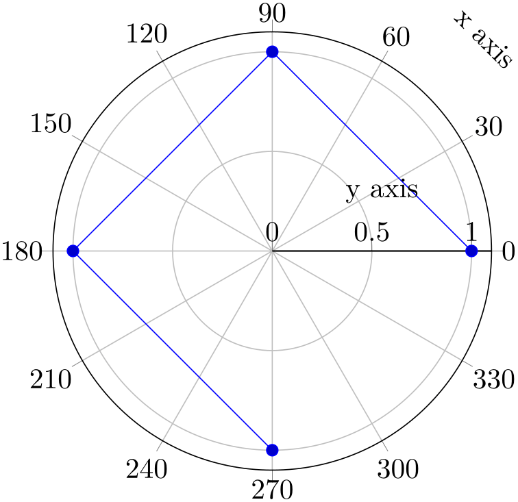
The polar library provides the polaraxis environment. Inside of such an environment, all coordinates are expected to be given in polar representation of the form \((\meta {angle},\meta {radius})\), i.e. the \(x\)-coordinate is always the angle and the \(y\)-coordinate the radius:
% Preamble: \pgfplotsset{width=7cm,compat=1.18}\usepgfplotslibrary{polar}
\begin{tikzpicture}
\begin{polaraxis}
                    \addplot coordinates
                {
(0,1)
(90,1)
(180,1)
(270,1)
};
\end{polaraxis}
\end{tikzpicture}
% Preamble: \pgfplotsset{width=7cm,compat=1.18}\usepgfplotslibrary{polar}
\begin{tikzpicture}
\begin{polaraxis}
\addplot+ [domain=0:3] (360*x,x); % (angle,radius)
\end{polaraxis}
\end{tikzpicture}

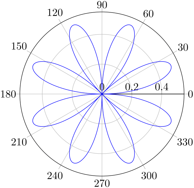
% Preamble: \pgfplotsset{width=7cm,compat=1.18}\usepgfplotslibrary{polar}
\begin{tikzpicture}
\begin{polaraxis}
\addplot+ [
mark=none,
domain=0:720,
samples=600,
]
{sin(2*x)*cos(2*x)};
% equivalent to (x,{sin(..)cos(..)}), i.e.
% the expression is the RADIUS
\end{polaraxis}
\end{tikzpicture}
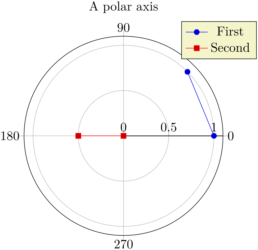
Polar axes support most of the pgfplots user interface, i.e. legend entries, any axis descriptions, xtick/ytick and so on:
% Preamble: \pgfplotsset{width=7cm,compat=1.18}\usepgfplotslibrary{polar}
\begin{tikzpicture}
\begin{polaraxis}[
xtick={0,90,180,270},
                    title=A
                polar axis,
]
                    \addplot coordinates
                {(0,1) (45,1)};
\addlegendentry{First}
                    \addplot coordinates
                {(180,0.5) (0,0)};
\addlegendentry{Second}
\end{polaraxis}
\end{tikzpicture}
Furthermore, you can use all of the supported input coordinate methods (like \addplot coordinates, \addplot table, \addplot expression). The only difference is that polar axes interpret the (first two) input coordinates as polar coordinates of the form \((\meta {angle in degrees},\meta {radius})\).
It is also possible to provide \addplot3; in this case, the third coordinate will be ignored (although it can be used as color data using point meta=z). An example can be found below in Section 5.10.3.
5.10.2Using Radians instead of Degrees
The initial configuration uses degrees for the angle (\(x\) component of every input coordinate). pgfplots also supports to provide the angle in radians using the data cs=polarrad switch:
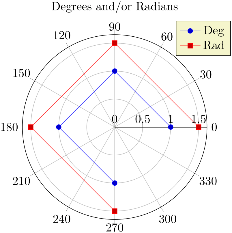
% Preamble: \pgfplotsset{width=7cm,compat=1.18}\usepgfplotslibrary{polar}
\begin{tikzpicture}
\begin{polaraxis}[title={Degrees and/or Radians}]
                    \addplot coordinates
                {
(0,1) (90,1) (180,1) (270,1)
};
\addlegendentry{Deg}
\addplot+ [
data cs=polarrad,
] coordinates {
(0,1.5) (pi/2,1.5)
(pi,1.5) (pi*3/2,1.5)
};
\addlegendentry{Rad}
\end{polaraxis}
\end{tikzpicture}
The data cs key is described in all detail on page (page for section 4.23); it tells pgfplots the coordinate system of input data. pgfplots will then take steps to automatically transform each coordinate into the required coordinate system (in our case, this is data cs=polar).
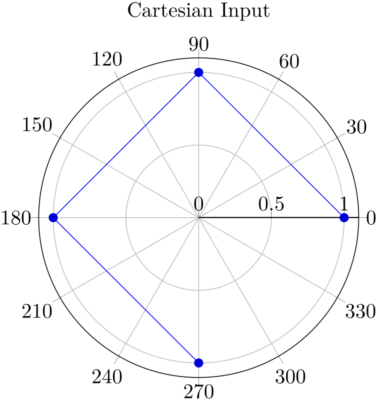
5.10.3Mixing With Cartesian Coordinates
Similarly to the procedure described above, you can also provide Cartesian coordinates inside of a polar axis: simply tell pgfplots that it should automatically transform them to polar representation by means of data cs=cart:
% Preamble: \pgfplotsset{width=7cm,compat=1.18}\usepgfplotslibrary{polar}
\begin{tikzpicture}
\begin{polaraxis}[title=Cartesian Input]
\addplot+ [
data cs=cart,
] coordinates {
(1,0) (0,1) (-1,0) (0,-1)
};
\end{polaraxis}
\end{tikzpicture}
More details about the data cs key can be found on page (page for section 4.23).
This does also allow more involved visualization techniques which may operate on Cartesian coordinates. The following example uses \addplot3 to sample a function \(f\colon \mathbb {R}^2 \to \mathbb {R}\), computes contour lines and displays the result in a polaraxis:
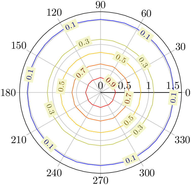
% Preamble: \pgfplotsset{width=7cm,compat=1.18}\usepgfplotslibrary{polar}
\begin{tikzpicture}
\begin{polaraxis}
\addplot3 [
contour lua,
domain=-3:3,
data cs=cart,
]
{exp(-x^2-y^2)};
\end{polaraxis}
\end{tikzpicture}
What happens is that \(z=\exp (-x^2-y^2)\) is sampled for \(x,y \in [-3,3]\), then contour lines are computed on \((x,y,z)\), then the resulting triples \((x,y,z)\) are transformed to polar coordinates \((\alpha ,r,z)\) (leaving \(z\) intact). Finally, the \(z\)-coordinate is used as point meta to determine the color.
Note that \addplot3 allows to process three-dimensional input types, but the result will always be two-dimensional (the \(z\)-coordinate is ignored for point placement in polaraxis). However, the \(z\)-coordinate can be used to determine point colors (using point meta=z).
5.10.4Polar Descriptions
Polar axes support axis labels just as other plot types.96 In this case, xticklabel cs refers to a label position for the angles (\(x\)-axis) and yticklabel cs refers to a label position for the radius (\(y\)-axis).
The default axis label for the angles is placed at \(45\) degrees,
% Preamble: \pgfplotsset{width=7cm,compat=1.18}\usepgfplotslibrary{polar}
\begin{tikzpicture}
\begin{polaraxis}[
                    xlabel=x
                axis,
                    ylabel=y
                axis,
]
                    \addplot coordinates
                {
(0,1) (90,1) (180,1) (270,1)
};
\end{polaraxis}
\end{tikzpicture}
and is configured as a sloped label using the default configuration
                    every axis
                x label/.style={
at={(xticklabel cs:0.125)},
sloped={at position=45},
anchor=near ticklabel,
near ticklabel at=45,
},
                    every axis
                y label/.style={
at={(yticklabel cs:0.5)},
anchor=near ticklabel,
},
This also allows sloped \(x\) labels as in the following example.97
% Preamble: \pgfplotsset{width=7cm,compat=1.18}\usepgfplotslibrary{polar}
\begin{tikzpicture}
\begin{polaraxis}[
                    xlabel=x
                axis,
                    ylabel=y
                axis,
xticklabel style={sloped like x axis},
]
                    \addplot coordinates
                {
(0,1) (90,1) (180,1) (270,1)
};
\end{polaraxis}
\end{tikzpicture}
96 Attention: support for polar axis labels is broken in versions before 1.13. Please upgrade to pgfplots 1.13 and use compat=1.13 or higher in order to use polar axis descriptions.
97 Note that sloped polar labels also requires pgfplots 1.13 and compat=1.13 or newer.
5.10.5Special Polar Plot Types
-
/tikz/polar comb(no value) 
-
\addplot+[polar comb]
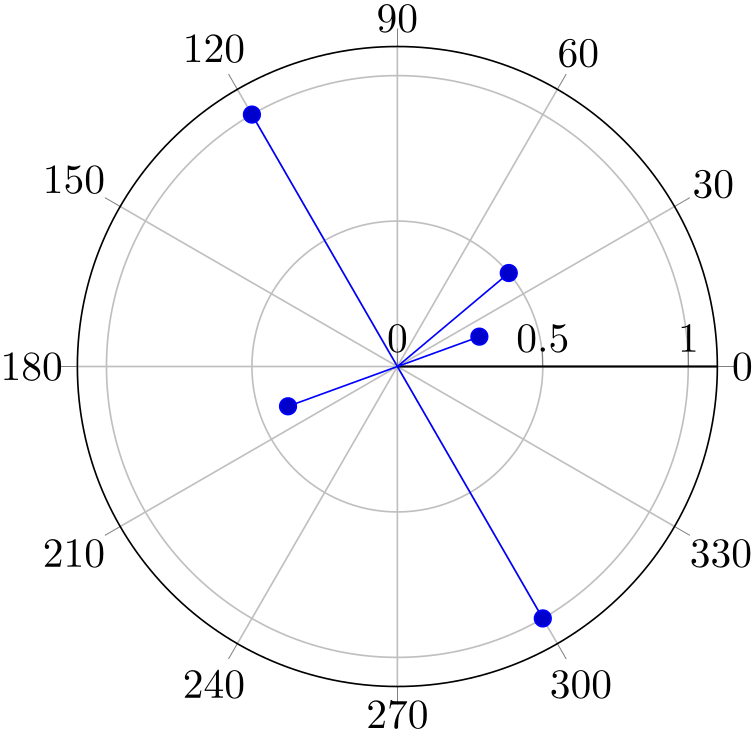
The polar comb plot handler is provided by TikZ; it draws paths from the origin to the designated position and places marks at the positions (similar to the comb plot handler). Since the paths always start at the origin, it is particularly suited for polaraxis:
% Preamble: \pgfplotsset{width=7cm,compat=1.18}\usepgfplotslibrary{polar}
\begin{tikzpicture}
\begin{polaraxis}
\addplot+ [
polar comb,
] coordinates {
(300,1)
(20,0.3)
(40,0.5)
(120,1)
(200,0.4)
};
\end{polaraxis}
\end{tikzpicture}
5.10.6Partial Polar Axes
The polar library also supports partial axes. If you provide xmin/xmax, you can restrict the angles used for the axis:
% Preamble: \pgfplotsset{width=7cm,compat=1.18}\usepgfplotslibrary{polar}
\begin{tikzpicture}
\begin{polaraxis}[
xmin=45,
xmax=360,
]
                    \addplot coordinates
                {
(0,1) (90,1) (180,1) (270,1)
};
\end{polaraxis}
\end{tikzpicture}
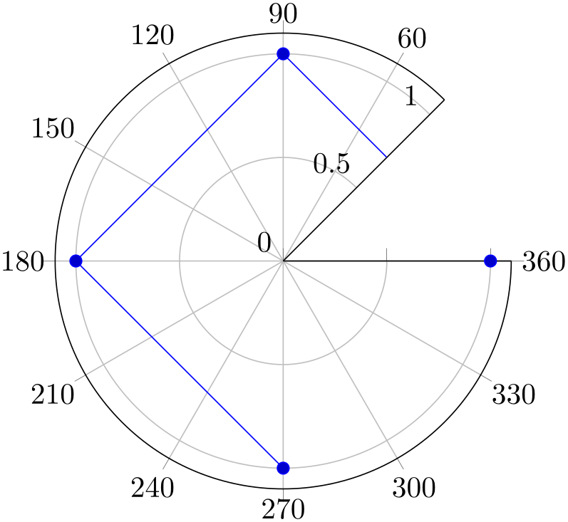
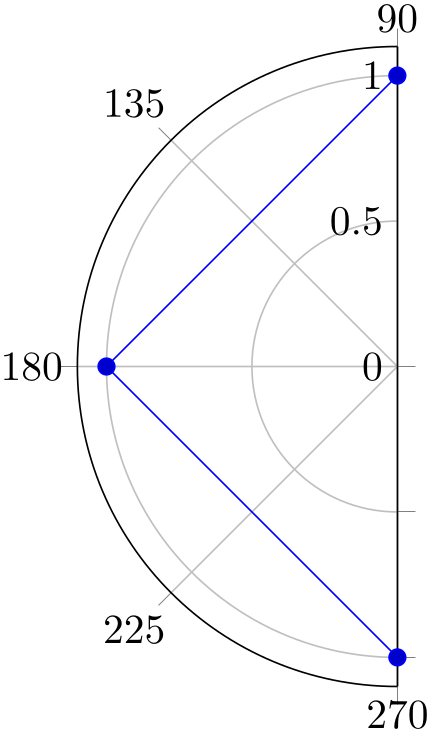
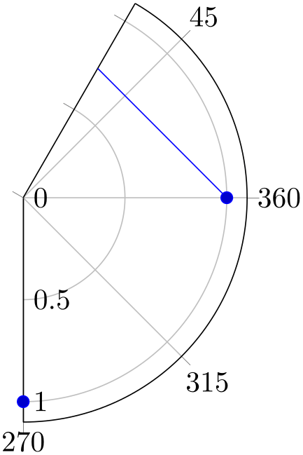
Currently, the first angle must be lower than the second one. But you can employ the periodicity to get pies as follows:
% Preamble: \pgfplotsset{width=7cm,compat=1.18}\usepgfplotslibrary{polar}
\begin{tikzpicture}
\begin{polaraxis}[xmin=90,xmax=270]
                        \addplot coordinates
                { (0,1) (90,1) (180,1) (270,1) };
\end{polaraxis}
\end{tikzpicture}~%
\begin{tikzpicture}
\begin{polaraxis}[xmin=270,xmax=420]
                        \addplot coordinates
                { (0,1) (90,1) (180,1) (270,1) };
\end{polaraxis}
\end{tikzpicture}
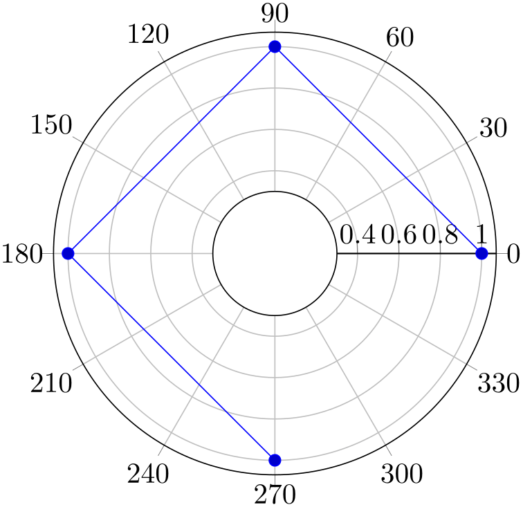
Similarly, an explicitly provided value for ymin allows to reduce the displayed range away from \(0\):
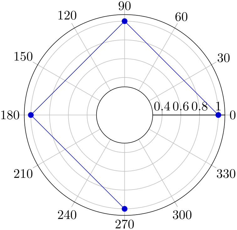
% Preamble: \pgfplotsset{width=7cm,compat=1.18}\usepgfplotslibrary{polar}
\begin{tikzpicture}
\begin{polaraxis}[
ymin=0.3,
]
                    \addplot coordinates
                {
(0,1) (90,1) (180,1) (270,1)
};
\end{polaraxis}
\end{tikzpicture}
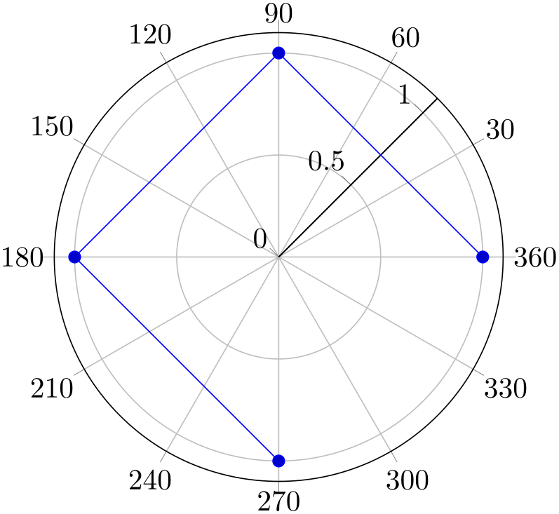
Modifying xmin and xmax manually can also be used to move the \(y\) axis line (the line with ytick and yticklabels):
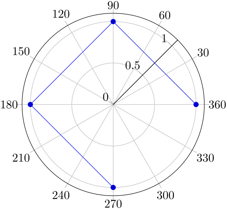
% Preamble: \pgfplotsset{width=7cm,compat=1.18}\usepgfplotslibrary{polar}
\begin{tikzpicture}
\begin{polaraxis}[
xmin=45,
xmax=405,
]
                    \addplot coordinates
                {
(0,1) (90,1) (180,1) (270,1)
};
\end{polaraxis}
\end{tikzpicture}