Manual for Package pgfplots
2D/3D Plots in LATeX, Version 1.18.2
https://github.com/pgf-tikz/pgfplots
The Reference
4.10Scaling Options
There are a various options which control or change the scaling of an axis. Here, “scaling” typically means two aspects: first, the unit vector size in each direction and second, the displayed limits in each direction. Both together control the size of the axis box. In addition, axis descriptions change the size. However, pgfplots scales only units and determines limits. It does not scale axis descriptions by default in order to keep consistent font sizes between the text and the figure.
Often, one wishes to provide the target size only and let pgfplots do the rest. This is the default; it scales the axis to width and height. If you provide one of these options, the axis will be rescaled while keeping the aspect ratio.
Occasionally, one wants to provide unit vectors explicitly to ensure that one unit takes a prescribed amount of space. This is possible by means of the x, y, and z keys. In such a case, the width and height options will be ignored (or only applied for the unspecified unit vectors).
Another common approach is to enforce specific unit vector ratios: for example by specifying that each unit should take the same amount of space using axis equal. Here, pgfplots scales the lengths of all vectors uniformly, i.e. it applies the same scale to each vector. This is done by means of the scale mode configuration which is basically one of scale mode=stretch to fill or scale mode=scale uniformly: pgfplots tries to satisfy the prescribed width and height arguments by finding a common scaling factor. In addition, it attempts to enlarge the limits individually to fit into the prescribed dimensions.
In addition, you can use the option /pgfplots/scale to simply scale all final units up by some prescribed factor. This does not change text labels.
If needed, you can also supply /tikz/scale to an axis. This will scale the complete resulting image, including all text labels.
4.10.1Common Scaling Options
All common options mentioned in the previous paragraphs are described here.
-
/pgfplots/width={
 dimen
dimen } (initially empty)
} (initially empty)
Sets the width of the final picture to {dimen}.
Any non-empty dimension like width=5cm sets the desired target width. Any TeX unit is accepted (like 200pt or 5in).
An empty value width={} means “use default width or rescale proportionally to height”. In this case, pgfplots uses the value of \axisdefaultwidth as target quantity. However, if the height key has been set, pgfplots will rescale the \axisdefaultwidth in a way which keeps the ratio between \axisdefaultwidth and \axisdefaultheight. This allows to specify just one of width and height and keep aspect ratios.
Consequently, if you specify just width=5cm but leave the default height={}, the scaling will respect the initial aspect ratio.
The scaling affects the unit vectors for \(x\), \(y\), and \(z\). It does not change the size of text labels or axis descriptions.
% Preamble: \pgfplotsset{width=7cm,compat=1.18}
\begin{tikzpicture}
\begin{axis}[
width=5cm,
]
\addplot {x};
\end{axis}
\end{tikzpicture}
Please note that pgfplots only estimates the size needed for axis- and tick labels. The estimate assumes a fixed amount of space for anything which is outside of the axis box. This has the effect that the final images may be slightly larger or slightly smaller than the prescribed dimensions. However, the fixed amount is always the same; it is set to 45pt. That means that multiple pictures with the same target dimensions will have the same size for their axis boxes – even if the size for descriptions varies.
It is also possible to scale the axis box to the prescribed width/height. In that case, the total width will be larger due to the axis descriptions. However, the axis box fills the desired dimensions exactly.
% Preamble: \pgfplotsset{width=7cm,compat=1.18}
\begin{tikzpicture}
\begin{axis}[
width=5cm,
scale only axis,
]
\addplot {x};
\end{axis}
\end{tikzpicture}
changing width and/or height changes only the unit vector sizes. In particular, it does not change the font size for any axis description, nor does it change the default spacing between adjacent tick labels. It is best practice to use width/height for “small” changes, i.e. changes for which the font size should remain the same. Consider using one of the styles normalsize, small, footnotesize, or tiny which are described in Section 4.10.2 on page (page for section 4.10.2), and then change to your desired dimensions if you need a different “quality” of scaling.
-
\axisdefaultwidth 
This macro defines the default width. It is preset to 240pt.
This default width defines the aspect ratio which will be used whenever just one of width or height is specified: the aspect ratio is the ratio between \axisdefaultwidth and \axisdefaultheight.
You can change it using
\def\axisdefaultwidth{10cm}
-
/pgfplots/height={
dimen} (initially empty)
-
\axisdefaultheight 
Works in the same way as width except that an empty value height={} defaults to “use either \axisdefaultheight or scale proportionally if just width has been changed”.
This macro defines the default height. It is preset to 207pt.
See \axisdefaultwidth.
-
/pgfplots/scale only axis=true|false (initially false) 
If scale only axis is enabled, width and height apply only to the axis rectangle. Consequently, the resulting figure is larger than width and height (because of any axis descriptions). However, the axis box has exactly the prescribed target dimensions.
If scale only axis=false (the default), pgfplots will try to produce the desired width including labels, titles and ticks.
-
/pgfplots/x={
dimen} (initially empty)
-
/pgfplots/y={
dimen} (initially empty)
-
/pgfplots/z={
dimen} (initially empty)
-
/pgfplots/x={(
x,y)}
-
/pgfplots/y={(
x,y)}
-
/pgfplots/z={(
x,y)}
Allows to assign zero, one, two, or three of the target unit vectors.
In this context, a “unit vector” is a two-dimensional vector which defines the projection onto the canvas: every logical plot coordinate \((x,y)\) is drawn at the canvas position
\(\seteqnumber{0}{}{0}\)\begin{equation*} x \cdot \begin{bmatrix} e_{xx} \\ e_{xy} \end {bmatrix} + y \cdot \begin{bmatrix} e_{yx} \\ e_{yy} \end {bmatrix}. \end{equation*}
The unit vectors \(e_x\) and \(e_y\) determine the paper position in the current (always two dimensional) image. For a standard three-dimensional axis, a plot coordinate \((x,y,z)\) is drawn at
\(\seteqnumber{0}{}{0}\)\begin{equation*} x \cdot \begin{bmatrix} e_{xx} \\ e_{xy} \end {bmatrix} + y \cdot \begin{bmatrix} e_{yx} \\ e_{yy} \end {bmatrix} + z \cdot \begin{bmatrix} e_{zx} \\ e_{zy} \end {bmatrix}. \end{equation*}
The initial setting assigns empty values to each of these keys, i.e. x={},y={},z={}. In this case, pgfplots is free to choose these vectors as best. To this end, it uses width, height, scale mode, plot box ratio, unit vector ratio, view, and the axis limits.
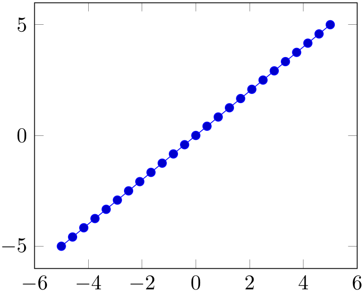
The key x={dimen} simply sets \(e_x = (\meta {dimen},0)^T \) while y={dimen} sets \(e_y = (0,\meta {dimen})^T\). Using z={dimen} results in \(e_z = (\meta {dimen},\meta {dimen})^T\). In this context,
dimen
is any
TeX
size like 1mm, 2cm or 5pt. Note that you should not use negative values for
dimen
(consider using x dir and its variants to
reverse axis directions).
% Preamble: \pgfplotsset{width=7cm,compat=1.18}
\begin{tikzpicture}
\begin{axis}[
x=1cm,
y=1cm,
]
                        \addplot expression
                    [domain=0:3] {2*x};
\end{axis}
\end{tikzpicture}
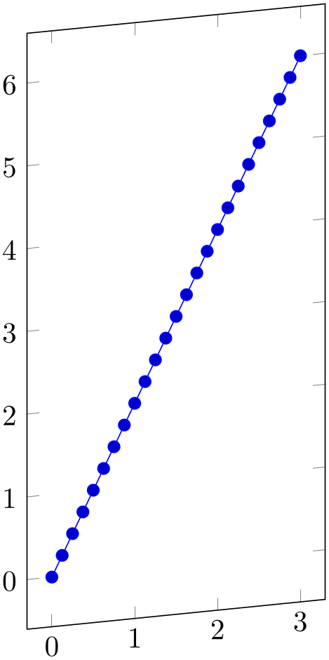
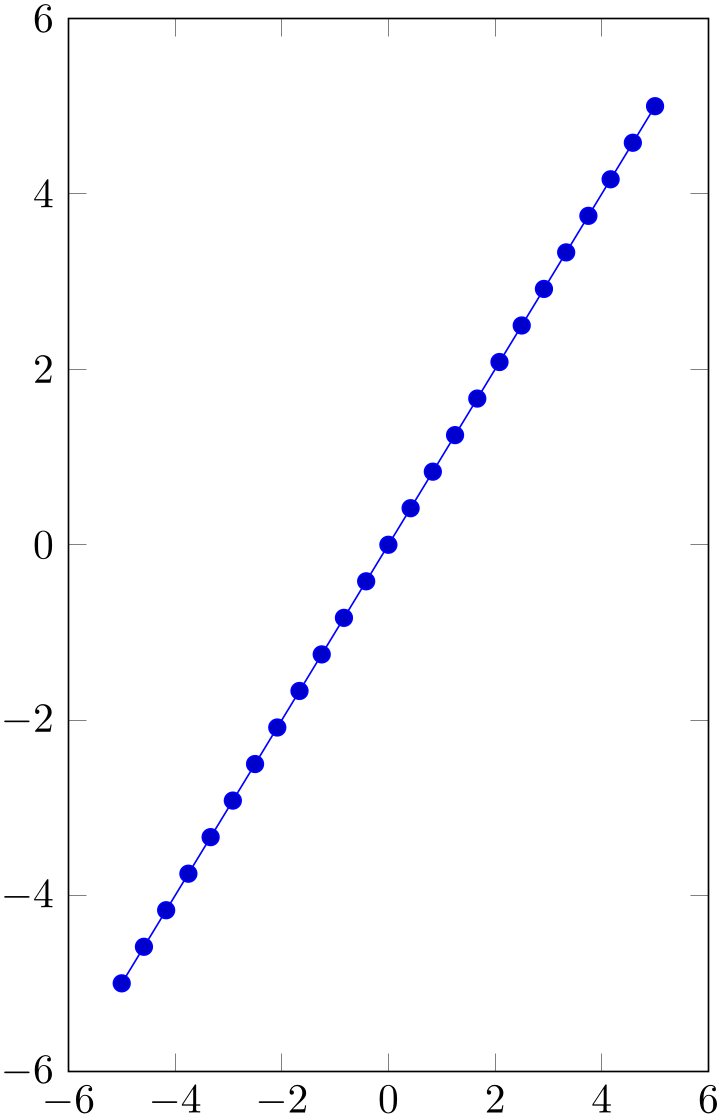
% Preamble: \pgfplotsset{width=7cm,compat=1.18}
\begin{tikzpicture}
\begin{axis}[
x=1cm,
y=0.5cm,
y dir=reverse,
]
                        \addplot expression
                    [domain=0:3] {2*x};
\end{axis}
\end{tikzpicture}
Note that if you change the unit vector for just one direction, the other vector(s) will be chosen by pgfplots – and scaled in order to fill the prescribed width and height as best as pgfplots can (but see remarks for three-dimensional plots at the end of this key).
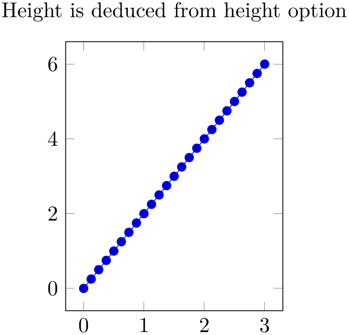
% Preamble: \pgfplotsset{width=7cm,compat=1.18}
\begin{tikzpicture}
\begin{axis}[
x=1cm,
                        title=Height is deduced from
                    height option,
]
                        \addplot expression
                    [domain=0:3] {2*x};
\end{axis}
\end{tikzpicture}
The second syntax, x={(x,y)} sets \(e_x = (\meta {x},\meta {y})^T\) explicitly.55 The
corresponding keys for y and
z work in a similar way. This allows to define skewed or
rotated axes.
% Preamble: \pgfplotsset{width=7cm,compat=1.18}
\begin{tikzpicture}
\begin{axis}[
x={(1cm,0.1cm)},
y=1cm,
]
                        \addplot expression
                    [domain=0:3] {2*x};
\end{axis}
\end{tikzpicture}
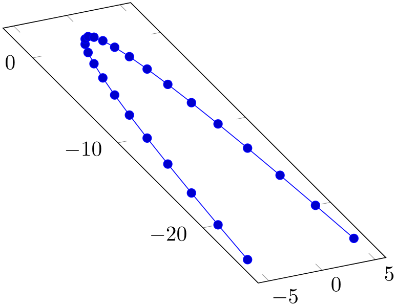
% Preamble: \pgfplotsset{width=7cm,compat=1.18}
\begin{tikzpicture}
\begin{axis}[
x={(5pt,1pt)},
y={(-4pt,4pt)},
]
\addplot {1-x^2};
\end{axis}
\end{tikzpicture}
Setting x and/or y for logarithmic axis will set the dimension used for \(1 \cdot e \approx 2.71828\) (or whatever has been set as log basis x).
Please note that it is not possible to specify x as argument to tikzpicture. The option
does not have any effect because an axis rescales its coordinates (see the width option).
Note that providing unit vectors explicitly usually causes pgfplots to ignore any other scaling options. In other words: if you say y=0.1cm, pgfplots will use \((0\text {cm},0.1\text {cm})\) as \(y\) projection vector. However, if you add scale mode=scale uniformly, you allow pgfplots to change the lengths of your vectors. Of course, it will keep their relative directions and relative sizes. In this case, pgfplots will try to determine a good common scaling factor and it will try to change the axis limits in order to fill the prescribed width and height (see the documentation for scale mode for details).
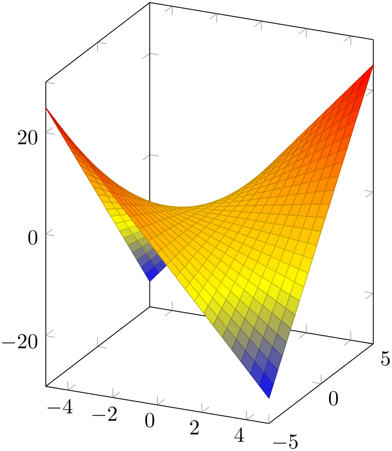
% Preamble: \pgfplotsset{width=7cm,compat=1.18}
\begin{tikzpicture}
\begin{axis}[
                        title=Allow to rescale
                    \emph{lengths},
x={(0.1cm,-0.05cm)},
y=0.1cm,
z=0cm,
axis on top,
scale mode=scale uniformly,
]
\addplot3 [surf,shader=interp] {x*y};
\end{axis}
\end{tikzpicture}
In the example above, pgfplots decided that it should only rescale units – at the expensive of the width constraint.
see also Section 4.10.2 if you want to change font sizes or the density of tick labels in a simple way.
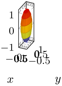
As of version 1.5, it is also possible to supply unit vectors to three-dimensional axes. In this case, the following extra assumptions need to be satisfied:
-
1. If you want to control three-dimensional units, you need to provide all of x, y, and z keys. For two-dimensional axes, it is also supported to supply just one of x or y.
-
2. Any provided three-dimensional unit vectors are assumed to form a right-handed coordinate system. In other words: take your right hand, let the thumb point into the x direction, the index finger in y direction and the middle finger in z direction. If that is impossible, the pgfplots output will be wrong. The reason for this assumption is that pgfplots needs to compute the view direction out of the provided units (see below).
Consider using x dir=reverse or its variants in case you want to reverse directions.
-
3. For three-dimensional axes, pgfplots computes a view direction out of the provided unit vectors. The view direction is required to allow the z buffer feature (i.e. to decide about depths).56
This feature is used to for the \addplot3 graphics feature, compare the examples in Section 4.3.8 on page (page for section 4.3.8).
-
/pgfplots/xmode=normal|linear|log (initially normal) 
-
/pgfplots/ymode=normal|linear|log (initially normal) 
-
/pgfplots/zmode=normal|linear|log (initially normal) 
Allows to choose between linear (=normal) or logarithmic axis scaling or log plots for each \(x,y,z\)-combination.
Logarithmic plots use the current setting of log basis x and its variants to determine the basis (default is \(e\)).
-
/pgfplots/axis equal={
true,false} (initially false)
Each unit vector is set to the same length while the axis dimensions stay constant. Afterwards, the size ratios for each unit in \(x\) and \(y\) will be the same.
Axis limits will be enlarged to compensate for the scaling effect.

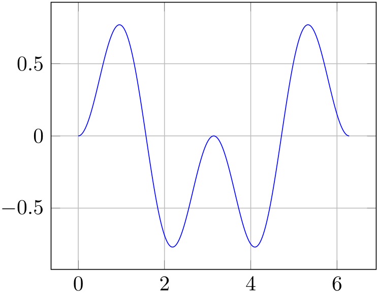
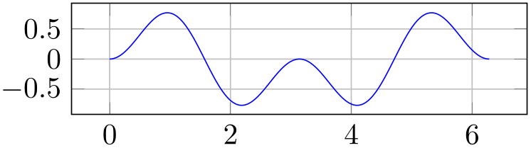
% Preamble: \pgfplotsset{width=7cm,compat=1.18}
\begin{tikzpicture}
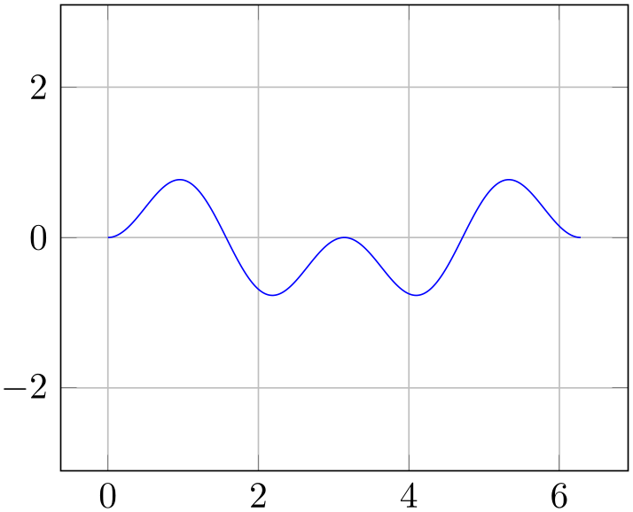
\begin{axis}[axis equal=false,grid=major]
                            \addplot [blue] expression
                    [domain=0:2*pi,samples=300] {sin(deg(x))*sin(2*deg(x))};
\end{axis}
\end{tikzpicture}
\hspace{1cm}
\begin{tikzpicture}
\begin{axis}[axis equal=true,grid=major]
                            \addplot [blue] expression
                    [domain=0:2*pi,samples=300] {sin(deg(x))*sin(2*deg(x))};
\end{axis}
\end{tikzpicture}
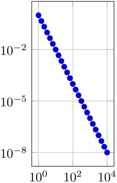
% Preamble: \pgfplotsset{width=7cm,compat=1.18}
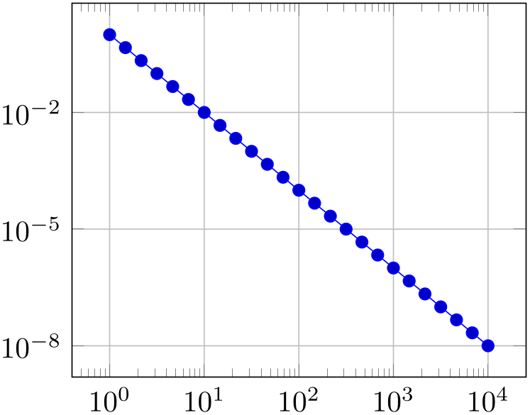
\begin{tikzpicture}
\begin{loglogaxis}[axis equal=false,grid=major]
\addplot expression [domain=1:10000] {x^-2};
\end{loglogaxis}
\end{tikzpicture}
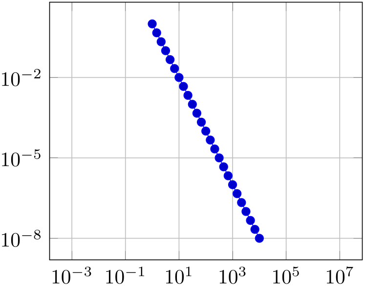
\hspace{1cm}
\begin{tikzpicture}
\begin{loglogaxis}[axis equal=true,grid=major]
\addplot expression [domain=1:10000] {x^-2};
\end{loglogaxis}
\end{tikzpicture}
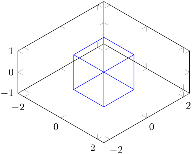
% Preamble: \pgfplotsset{width=7cm,compat=1.18}
\begin{tikzpicture}
\begin{axis}[axis equal,small,view={45}{35.26}]
\addplot3 [mark=cube, blue, mark size=1cm]
                            coordinates
                    {(0,0,0)};
\end{axis}
\end{tikzpicture}
The configuration axis equal=true is actually just a style which sets unit vector ratio=1 1 1,unit rescale keep size=true.
-
/pgfplots/axis equal image={
true,false} (initially false)
Similar to axis equal, but the axis limits will stay constant as well (leading to smaller images).
% Preamble: \pgfplotsset{width=7cm,compat=1.18}
\begin{tikzpicture}
\begin{axis}[axis equal image=false,grid=major]
                            \addplot [blue] expression
                    [domain=0:2*pi,samples=300] {sin(deg(x))*sin(2*deg(x))};
\end{axis}
\end{tikzpicture}
\hspace{1cm}
\begin{tikzpicture}
\begin{axis}[axis equal image=true,grid=major]
                            \addplot [blue] expression
                    [domain=0:2*pi,samples=300] {sin(deg(x))*sin(2*deg(x))};
\end{axis}
\end{tikzpicture}

% Preamble: \pgfplotsset{width=7cm,compat=1.18}
\begin{tikzpicture}
\begin{loglogaxis}[axis equal image=false,grid=major]
\addplot expression [domain=1:10000] {x^-2};
\end{loglogaxis}
\end{tikzpicture}
\hspace{1cm}
\begin{tikzpicture}
\begin{loglogaxis}[axis equal image=true,grid=major]
\addplot expression [domain=1:10000] {x^-2};
\end{loglogaxis}
\end{tikzpicture}
The configuration axis equal image=true is actually just a style which sets unit vector ratio=1 1 1,unit rescale keep size=false.
-
/pgfplots/unit vector ratio={
rx ry rz} (initially empty)
-
/pgfplots/unit vector ratio*={
rx ry rz}
-
/pgfplots/unit rescale keep size=true|false|unless limits declared (initially unless limits declared) 
Allows to provide custom unit vector ratios.
The key allows to tell pgfplots that, for example, one unit in \(x\) direction should be twice as long as one unit in \(y\) direction:
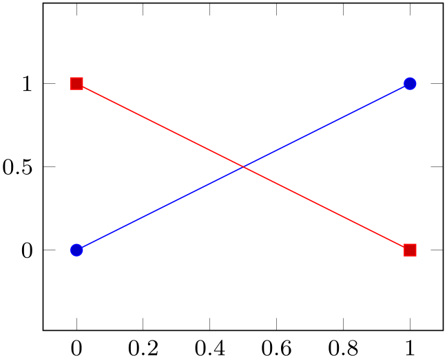
% Preamble: \pgfplotsset{width=7cm,compat=1.18}
\begin{tikzpicture}
\begin{axis}[unit vector ratio=2 1,small]
                        \addplot coordinates
                    {(0,0) (1,1)};
                        \addplot table
                    [row sep=\\,col sep=&] {
                            x &
                    y \\
0 & 1 \\
1 & 0 \\
};
\end{axis}
\end{tikzpicture}
Providing unit vector ratio=2 1 means that \(\frac {||e_x||}{||e_y||} = 2\) where each coordinate \((x,y)\) is placed at \(x e_x + y e_y \in \mathbb {R}^2\) (see the documentation for x and y options). Note that axis equal is nothing but unit vector ratio=1 1 1.
The arguments
rx,
ry, and
rz
are ratios for \(x\), \(y\) and \(z\) vectors, respectively. For two-dimensional axes, only
rx
and
ry
are considered; they are provided relative to the \(y\)-axis. In other words: the \(x\) unit vector will be
rx\(/\)ry
times longer than the \(y\) unit vector. For three-dimensional axes, all three arguments can be provided; they are
interpreted relative to the \(z\) unit vector. Thus, a three dimensional axis with
unit vector ratio=1 2 4 will have an \(x\) unit
which is \(\nicefrac 14\) the length of the \(z\) unit, and a \(y\) unit which is \(\nicefrac 24\) the length of the \(z\)
unit.
Trailing values of 1 can be omitted, i.e. unit vector ratio=2 1 is the same as unit vector ratio=2; and unit vector ratio=3 2 1 is the same as unit vector ratio=3 2. An empty value unit vector ratio={} disables unit vector rescaling.
Note that an active unit vector ratio will implicitly set scale mode=scale uniformly.57
In the default configuration, pgfplots maintains the original axis dimensions even though unit vector ratio involves different scalings.
It does so by enlarging the limits.
% Preamble: \pgfplotsset{width=7cm,compat=1.18}
\begin{tikzpicture}
\begin{axis}[footnotesize,xlabel=$x$,ylabel=$y$,unit vector ratio=]
\addplot3 [surf,z buffer=sort,samples=15,
variable=\u, variable y=\v,
domain=0:180, y domain=0:360]
                                       ({cos(u)*sin(v)},
                        {sin(u)*sin(v)}, {cos(v)});
\end{axis}
\end{tikzpicture}
\begin{tikzpicture}
\begin{axis}[footnotesize,xlabel=$x$,ylabel=$y$,unit vector ratio=1 1 1]
\addplot3 [surf,z buffer=sort,samples=15,
variable=\u, variable y=\v,
domain=0:180, y domain=0:360]
                                       ({cos(u)*sin(v)},
                        {sin(u)*sin(v)}, {cos(v)});
\end{axis}
\end{tikzpicture}
\begin{tikzpicture}
\begin{axis}[footnotesize,xlabel=$x$,ylabel=$y$,unit vector ratio=0.25 0.5]
\addplot3 [surf,z buffer=sort,samples=15,
variable=\u, variable y=\v,
domain=0:180, y domain=0:360]
                                       ({cos(u)*sin(v)},
                        {sin(u)*sin(v)}, {cos(v)});
\end{axis}
\end{tikzpicture}
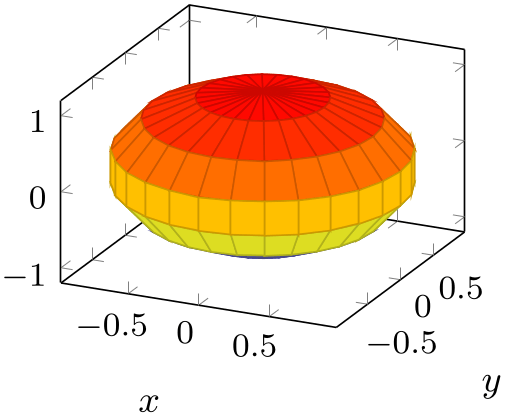
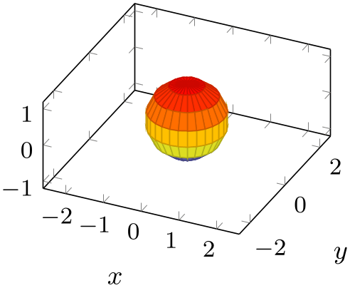
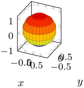
The example above has the same plot, with three different unit ratios. The first has no limitations (it is the default configuration). The second uses the same length for each unit vector and enlarges the limits in order to maintain the same dimensions. The third example has an \(x\) unit which is \(\nicefrac 14\) the length of a \(z\) unit, and an \(y\) unit which is \(\nicefrac 12\) the length of a \(z\) unit.
pgfplots does its best to respect the involved scaling options (the prescribed width and height, the unit vector ratio, and any specified axis limits). In the case above, it enlarged the horizontal limits and kept the \(z\) limit as is. See scale mode and its documentation for details about the involved algorithm and its parameters.
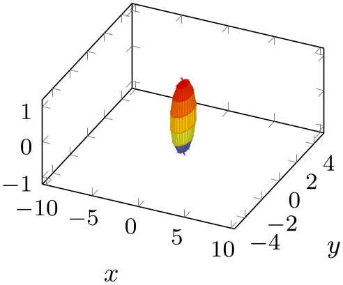
The unit rescale keep size=false key, or, equivalently, unit vector ratio*=..., does not enlarge limits:

% Preamble: \pgfplotsset{width=7cm,compat=1.18}
\begin{tikzpicture}
\begin{axis}[footnotesize,xlabel=$x$,ylabel=$y$,unit vector ratio=]
\addplot3 [surf,z buffer=sort,samples=15,
variable=\u, variable y=\v,
domain=0:180, y domain=0:360]
                                       ({cos(u)*sin(v)},
                        {sin(u)*sin(v)}, {cos(v)});
\end{axis}
\end{tikzpicture}
\begin{tikzpicture}
\begin{axis}[footnotesize,xlabel=$x$,ylabel=$y$,
unit rescale keep size=false,
unit vector ratio=1 1 1]
\addplot3 [surf,z buffer=sort,samples=15,
variable=\u, variable y=\v,
domain=0:180, y domain=0:360]
                                       ({cos(u)*sin(v)},
                        {sin(u)*sin(v)}, {cos(v)});
\end{axis}
\end{tikzpicture}
\begin{tikzpicture}
\begin{axis}[footnotesize,xlabel=$x$,ylabel=$y$,
unit vector ratio*=0.25 0.5, % the '*' implies 'unit rescale keep size=false'
]
\addplot3 [surf,z buffer=sort,samples=15,
variable=\u, variable y=\v,
domain=0:180, y domain=0:360]
                                       ({cos(u)*sin(v)},
                        {sin(u)*sin(v)}, {cos(v)});
\end{axis}
\end{tikzpicture}
The key unit rescale keep size also affects scale mode=scale uniformly (which is closely related to axis equal).
Here is the reference of the value of unit rescale keep size: the value true means that pgfplots will enlarge limits in order to keep the size. It will try to respect user provided limits, but if the user provided all limits, it will override the user-provided limits and will rescale them. Thus, true gives higher priority to the axis size than to user-provided limits. The choice false will never rescale axis limits. The choice unless limits declared is a mixture: it will enlarge limits unless the user provided them. If the user provides all limits explicitly, this choice is the same as false.
-
/pgfplots/x post scale={
scale} (initially empty)
-
/pgfplots/y post scale={
scale} (initially empty)
-
/pgfplots/z post scale={
scale} (initially empty)
-
/pgfplots/scale={
scale} (initially empty)
Lets pgfplots compute the axis
scaling based on width, height, view, plot box ratio, axis equal or explicit unit vectors with
x, y, z and rescales the resulting vector(s)
according to
scale.
The scale key sets all three keys to the same
uniform scale
value. This is effectively the same as if you rescale the complete axis (without changing sizes of descriptions).
The other keys allow individually rescaled axes.
% Preamble: \pgfplotsset{width=7cm,compat=1.18}
\begin{tikzpicture}
\begin{axis}[y post scale=1]
\addplot {x};
\end{axis}
\end{tikzpicture}
\begin{tikzpicture}
\begin{axis}[y post scale=2]
\addplot {x};
\end{axis}
\end{tikzpicture}
Thus, the axis becomes larger. This overrules any previous scaling.
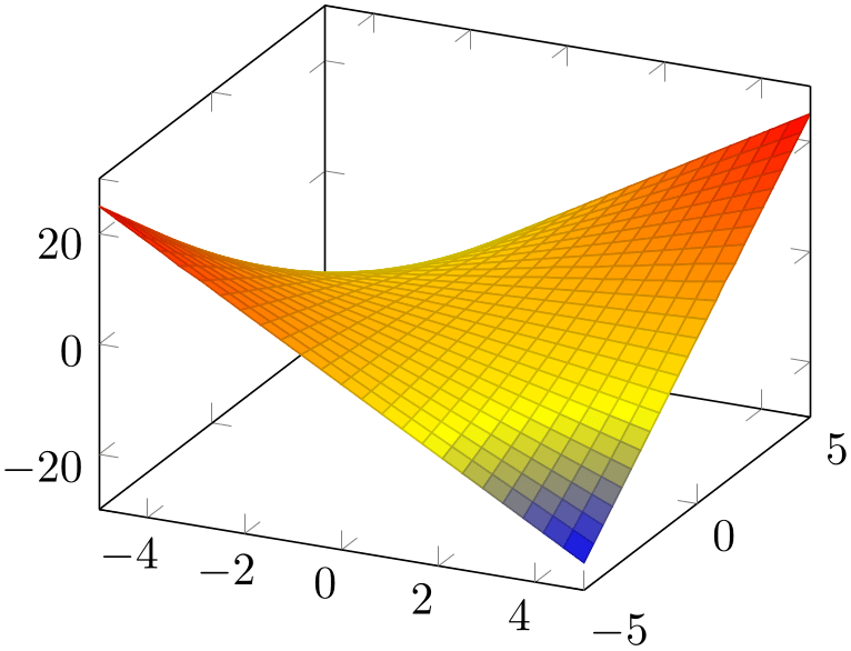
% Preamble: \pgfplotsset{width=7cm,compat=1.18}
\begin{tikzpicture}
\begin{axis}[z post scale=1]
                            \addplot3
                    [surf] {x*y};
\end{axis}
\end{tikzpicture}
\begin{tikzpicture}
\begin{axis}[z post scale=2]
                            \addplot3
                    [surf] {x*y};
\end{axis}
\end{tikzpicture}
55 Please note that you need extra curly braces around the vector. Otherwise, the comma will be interpreted as separator for the next key–value pair.
56 pgfplots provides a debug option called
view dir={ x
x }{y}{z}
to override the view direction, should that ever be interesting.
}{y}{z}
to override the view direction, should that ever be interesting.
57 This has been introduced in version 1.6. For older versions, the axis equal feature produced wrong results for three-dimensional axes.
4.10.2Scaling Descriptions: Predefined Styles
It is reasonable to change font sizes, marker sizes etc. together with the overall plot size: Large plots should also have larger fonts and small plots should have small fonts and a smaller distance between ticks.
-
/tikz/font=\normalfont|\small|\tiny|\(\dotsc \) 
-
/pgfplots/max space between ticks={
integer}
-
/pgfplots/try min ticks={
integer}
-
/tikz/mark size={
integer}
These keys should be adjusted to the figure’s dimensions. Use
\pgfplotsset{
tick label style={font=\footnotesize},
label style={font=\small},
legend style={font=\small},
}
to provide different fonts for different descriptions.
The keys max space between ticks and try min ticks are described on page (page for section 4.15.4) and configure the approximate distance and number of successive tick labels (in pt). Please omit the pt suffix here.
There are a couple of predefined scaling styles which set some of these options:
-
/pgfplots/normalsize(style, no value) 
Reinitializes the standard scaling options of pgfplots.
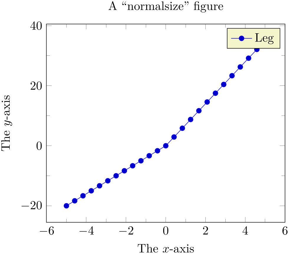
% Preamble: \pgfplotsset{width=7cm,compat=1.18}
\begin{tikzpicture}
\begin{axis}[normalsize,
title=A ``normalsize'' figure,
xlabel=The $x$-axis,
ylabel=The $y$-axis,
minor tick num=1,
legend entries={Leg},
]
\addplot {max(4*x,7*x)};
\end{axis}
\end{tikzpicture}
The initial setting is
\pgfplotsset{
normalsize/.style={
/pgfplots/width=240pt,
/pgfplots/height=207pt,
/pgfplots/max space between ticks=35,
},
}
-
/pgfplots/small(style, no value) 
Redefines several keys such that the axis is “smaller”.
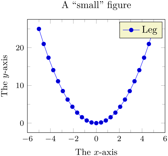
% Preamble: \pgfplotsset{width=7cm,compat=1.18}
\begin{tikzpicture}
\begin{axis}[
small,
title=A ``small'' figure,
xlabel=The $x$-axis,
ylabel=The $y$-axis,
minor tick num=1,
legend entries={Leg},
]
\addplot {x^2};
\end{axis}
\end{tikzpicture}
The initial setting is
\pgfplotsset{
small/.style={
width=6.5cm,
height=,
tick label style={font=\footnotesize},
label style={font=\small},
max space between ticks=25,
},
}
Feel free to redefine the scaling – the option may still be useful to get more ticks without typing too much. You could, for example, set small,width=6cm.
-
/pgfplots/footnotesize(style, no value) 
Redefines several keys such that the axis is even smaller. The tick labels will have \footnotesize.
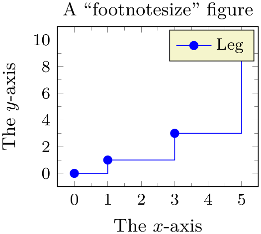
% Preamble: \pgfplotsset{width=7cm,compat=1.18}
\begin{tikzpicture}
\begin{axis}[
footnotesize,
                        title=A ``footnotesize''
                    figure,
xlabel=The $x$-axis,
ylabel=The $y$-axis,
minor tick num=1,
legend entries={Leg},
]
\addplot+ [const plot] coordinates {
(0,0) (1,1) (3,3) (5,10)
};
\end{axis}
\end{tikzpicture}
The initial setting is
\pgfplotsset{
footnotesize/.style={
width=5cm,
height=,
legend style={font=\footnotesize},
tick label style={font=\footnotesize},
label style={font=\small},
title style={font=\small},
every axis title shift=0pt,
max space between ticks=15,
every mark/.append style={mark size=8},
major tick length=0.1cm,
minor tick length=0.066cm,
},
}
As for small, it can be convenient to set footnotesize and set width afterwards.
You will need compat=1.3 or newer for this to work.
-
/pgfplots/tiny(style, no value) 
Redefines several keys such that the axis is very small. Most descriptions will have \tiny as fontsize.
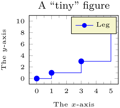
% Preamble: \pgfplotsset{width=7cm,compat=1.18}
\begin{tikzpicture}
\begin{axis}[tiny,
title=A ``tiny'' figure,
xlabel=The $x$-axis,
ylabel=The $y$-axis,
minor tick num=1,
legend entries={Leg},
]
\addplot+ [const plot] coordinates {
(0,0) (1,1) (3,3) (5,10)
};
\end{axis}
\end{tikzpicture}
The initial setting is
\pgfplotsset{
tiny/.style={
width=4cm,
height=,
legend style={font=\tiny},
tick label style={font=\tiny},
label style={font=\tiny},
title style={font=\footnotesize},
every axis title shift=0pt,
max space between ticks=12,
every mark/.append style={mark size=6},
major tick length=0.1cm,
minor tick length=0.066cm,
every legend image post/.append style={scale=0.8},
},
}
As for small, it can be convenient to use tiny,width=4.5cm to adjust the width.
You will need compat=1.3 or newer for this to work.
4.10.3Scaling Strategies
The content of this section is quite involved – and its knowledge is typically unnecessary because by default, pgfplots controls the involved stuff automatically. You may want to skip this section.
-
/pgfplots/scale mode=auto|none|stretch to fill|scale uniformly (initially auto) 
-
/pgfplots/scale uniformly strategy=auto|units only|change vertical limits|
change horizontal limits (initially auto) 
Specifies how to choose the (individual) unit vector scaling factors, their length ratios, and perhaps the axis limits in order to fill the prescribed width and height.
The scale mode implementation expects some “initial” set of unit vectors. This initial set of unit vectors is determined as follows: for standard two-dimensional axes, it is simply the unit cube \(e_x=(1\text {pt},0\text {pt})^T\), \(e_y=(0\text {pt},1\text {pt})^T\), \(e_z=0\). For three-dimensional axes, it is the outcome of the two keys view and plot box ratio. If you provided units explicitly by means of one of x, y, or z, this value is the initial unit vector.
In addition, it expects “initial” axis limits (i.e. values of xmin, xmax, etc.). The initial axis limits are those limits which have been deduced from your data or which have been provided explicitly. Furthermore, the initial axis limits already include changes of the enlargelimits key.
Given the initial set of unit vectors and the initial axis limits, the scale mode implementation is a kind of “post-processor” which creates modified unit vectors and modified axis limits in order to satisfy all specified constraints. These constraints are width, height, and unit vector ratio.
The initial choice auto tells pgfplots to take full control over this key. It chooses one of the other possible choices depending on the actual context. The choice auto evaluates to scale uniformly if unit vector ratio is set. Otherwise it evaluates to stretch to fill.
The choice none does not apply any rescaling at all. Use this if prescribed lengths of x, y (and perhaps z) should be used. In other words: it ignores width and height. In this case, you may want to set x post scale and its variants to rescale units manually. See also disabledatascaling.
The choice stretch to fill takes the initial unit vectors and rescales the unit vectors with two separate scales: one which results in the proper width and one which results in the proper height. As a consequence, the unit vectors are modified and distorted such that the final image fits into the prescribed dimensions. This is usually what one expects unless one provides unit directions explicitly. This mode does not change axis limits. Note that if one of the unit vectors has been provided explicitly, pgfplots will not change it. It will only change the remaining axis limits. This mode contradicts axis equal or unit vector ratio.
The choice scale uniformly takes the initial unit vectors and applies only one scaling factor to all units. In this case, there is just one common scaling factor for both width and height. Naturally, this will result in unsatisfactory results because either the final width or the final height will not be met. Therefore, this choice will adjust axis limits to get the desired dimensions. Thus, the unit vectors have exactly the same size relations and angles as they had before the scaling; only their magnitude is changed uniformly. In addition, axis limits may be changed (with individual scaling factors for each axis limit). Note that if unit vectors have been provided explicitly, pgfplots can still rescale it with this choice – it will keep the relative directions and size ratios. The choice scale uniformly tries its best to modify the degrees of freedom in a “useful” way. The precise meaning of “useful” is the scale uniformly strategy key.
The scale uniformly method requires to determine one common scaling factor which rescales every axis unit. In addition, it allows one scaling factor for each axis limit, i.e. up to three.
The constraints for this search are that we want to satisfy the width/height constraint, have as few rescaling as possible and that we do not want to reduce limits (as this could possibly hide data points).
The choice auto chooses one of the other possibilities automatically. Depending on whether we have two dimensions or three dimensions, it compares the available methods and chooses the one which does not reduce limits and which involves the fewest rescaling (i.e. it may compare the outcome of the other strategies). This is the default. If you keep the choice auto, you do not have to worry about the remaining choices. Note that manually provided axis limits will not be modified.
The choice units only will not enlarge axis limits. It will only rescale the units. To this end, it chooses the scaling factor such that the smaller target dimension is filled as desired. In other words: if width \(<\) height, it will scale to satisfy the width constraint. The height constraint will be ignored. The case \(>\) will be done the other way round. The choice units only typically results in a square axis as it takes the initial set of unit vectors (which are typically the unit box) and scales them with a common scaling factor. Consequently, you can choose units only if you want a boxed axis. You can still change axis limits manually, however.
The choice change vertical limits chooses a common scaling factor for the unit vectors on order to satisfy the width (!) constraint. This common scaling factor is similar to units only – but units only can also decide to satisfy the height constraint whereas change vertical limits will scale unit vectors to satisfy width. In order to satisfy the height constraint, change vertical limits modifies just the vertical limits. For two-dimensional axes, this is ymin and ymax. For three-dimensional axes, this is zmin and zmax. Clearly, there is a chance that it will decrease the displayed range – in this case, parts of the image will be clipped away. This method assumes that the vertical axis has not been rotated (i.e. that \(e_{yx}=0\) or \(e_{zx}=0\), respectively). It refuses to work and falls back to units only for rotates axes. Choose change vertical limits if you want the image (i.e. the actual content) as wide as possible. You can modify width and height to improve its outcome. Note that manually specified axis limits will not be changed, see below for details.
The choice change horizontal limits attempts a similar approach, but for the horizontal limits: it determines one suitable scaling factor which is applied to all unit vectors and modifies horizontal axis limits to satisfy the remaining constraints. For two-dimensional axes, this is quite simple because we typically have \(e_{xy} = 0\) (i.e. the \(x\) unit vector has vanishing \(y\) component) and \(e_{yx}=0\) such that pgfplots can change axis limits easily. If a two-dimensional axis has an \(x\) unit with \(e_{xy} \neq 0\), the method is not applicable and falls back to units only. For three-dimensional axes, it assumes that the \(z\) vector is not rotated, i.e. \(e_{zy} = 0\) and tries to change limits for both \(x\) and \(y\). This choice is much more involved because here, \(x\) and \(y\) components are coupled. Consequently, the common unit scaling factor and the two involved axis limit compensation factors for \(x\) and \(y\) are tightly coupled as well. pgfplots solves a system of nonlinear equations iteratively to arrive at a suitable solution for all three scalings. Use this method if change vertical limits would clip away parts of the image (because it reduced the displayed range) and you do not want to change width and height. The choice change horizontal limits will typically result in more empty space in the resulting figure. But it will not clip away content. Manually specified axis limits will not be changed, see below for details.
Manually provided axis limits:
Any manually provided arguments for xmin and its variants are considered to be immutable; pgfplots will not change them. If you assign xmin, pgfplots will only change xmax and vice versa. If you assign both xmin and xmax, pgfplots will not change \(x\) limits at all. Note that if you assign both xmin and xmax, pgfplots will simply skip the scaling and will give up on the constraints. It will not try to compensate the lack of scaling opportunities by changing \(y\) limits, for example. This has the positive effect that assigning limits does not change the complete appearance of your axis. The allowed set of changes to axis limits can be configured with the following key.
Interaction with enlargelimits:
Note that enlargelimits and scale mode are independent of another: the outcome of enlargelimits is used as “initial axis limits” and these limits may be changed by scale mode (even if you said enlargelimits=false). See the documentation of enlargelimits for details on this interaction.
-
/pgfplots/unit rescale keep size=true|false|unless limits declared (initially unless limits declared)
In the default configuration unless limits declared, unit rescaling may cause changes to the axis limits in order to keep the figure’s size intact. However, only those limits which have not been declared manually are subject to rescaling: if you say xmin=1, only xmax and the limits for \(y\) and \(z\) are free to change.
Setting unit rescale keep size=false will disable the modification of axis limits altogether, i.e. axis limits will not be rescaled to compensate scalings on unit vectors.
Setting unit rescale keep size=true will always rescale limits, even if they have been declared manually.
This key mainly affects scale mode=scale uniformly. This, in turn, is used for axis equal and \addplot3 graphics.
See also the addition documentation for this key and related examples on page (page for section 4.10.1).
The scale uniformly choice is implicitly used for axis equal and for the \addplot3 graphics feature, see the documentation in Section 4.3.8 on page (page for section 4.3.8) for its examples. Note that the common case is that the initial unit vectors form the unit cube (i.e. those before scaling, see above). In this case, scale uniformly is the same as axis equal.