Manual for Package pgfplots
2D/3D Plots in LATeX, Version 1.18.2
https://github.com/pgf-tikz/pgfplots
The Reference
4.24Fitting Lines – Regression
This section documents the attempts of pgfplots to fit lines to input coordinates. pgfplots currently supports create col/linear regression applied to columns of input tables. The feature relies on PgfplotsTable, it is actually implemented as a table postprocessing method.
-
/pgfplots/table/create col/linear regression={
 key-value-config
 }
}
-
/pgfplots/table/create col/linear regression/table={
 \macro or file name
 } (initially empty)
-
/pgfplots/table/create col/linear regression/x={
 column
 } (initially empty)
-
/pgfplots/table/create col/linear regression/y={
 column
 } (initially empty)
-
/pgfplots/table/create col/linear regression/xmode=auto|linear|log (initially auto) 
-
/pgfplots/table/create col/linear regression/ymode=auto|linear|log (initially auto) 
-
/pgfplots/table/create col/linear regression/variance list={
 list
list } (initially empty)
-
/pgfplots/table/create col/linear regression/variance={
 column name
 } (initially empty)
-
/pgfplots/table/create col/linear regression/variance src={
 \table or file name
 } (initially empty)
-
/pgfplots/table/create col/linear regression/variance format=linear|log (initially log) 
A style
for use in
\addplot table
which computes a linear (least squares) regression \(y(x) = a \cdot x + b\) using the sample data \((x_i,y_i)\) which has to
be specified inside of
 key-value-config
 (see below).
It creates a new column on the fly which contains the values \(y(x_i) = a \cdot x_i + b\). The values \(a\) and \(b\) will be stored (globally) into \pgfplotstableregressiona and \pgfplotstableregressionb.

% Preamble: \pgfplotsset{width=7cm,compat=1.18}
\begin{tikzpicture}
\begin{axis}[legend pos=outer north east]
\addplot table {% plot X versus Y. This is original data.
X Y
1 1
2 4
3 9
4 16
5 25
6 36
};
\addplot table [
y={create col/linear regression={y=Y}}, % compute a linear regression from the input table
] {
X Y
1 1
2 4
3 9
4 16
5 25
6 36
};
                            % \xdef\slope{\pgfplotstableregressiona} %<-- might be handy
                    occasionally
\addlegendentry{$y(x)$}
\addlegendentry{%
$\pgfmathprintnumber{\pgfplotstableregressiona} \cdot x
\pgfmathprintnumber[print sign]{\pgfplotstableregressionb}$}
\end{axis}
\end{tikzpicture}
The example above has two plots: one showing the data and one containing the linear regression line. We use
y={create col/linear regression={}} here, which means to create a
new column73 containing the regression values automatically. As arguments, we
need to provide the \(y\) column name explicitly.74 The \(x\) value is determined from context:
linear regression is evaluated inside of
\addplot table, so it uses the same \(x\) as
\addplot table
(i.e. if you write \addplot table[x={ col name
 }], the regression will also use
 col name
 as its x input). Furthermore, it shows the line parameters \(a\) and
\(b\) in the legend.
Note that the uncommented line with \xdef\slope{\pgfplotstableregressiona} is useful if you have more than one regression line: it copies the value of \pgfplotstableregressiona (in this case) into a new global variable called ‘\slope’. This allows to use ‘\slope’ instead of \pgfplotstableregressiona – even after \pgfplotstableregressiona has been overwritten.
The following
 key-value-config
 keys are accepted as comma-separated list:
Provides the table from where to load the x and y columns. It defaults to the currently processed one, i.e. to the value of \pgfplotstablename.
Provides the source of \(x_i\) and \(y_i\) data, respectively. The argument
 column
 is usually a column name of the input table, yet it can also contain [index]
 integer
 to designate column indices (starting with \(0\)),
create on use specifications or
aliases (see the PgfplotsTable manual for details on
create on use and
alias).
The initial configuration (an empty value) checks the context where the linear regression is evaluated. If it is evaluated inside of \pgfplotstabletypeset, it uses the first and second table columns. If it is evaluated inside of \addplot table, it uses the same \(x\) input as the \addplot table statement. The y key needs to be provided explicitly (unless the table has only two columns).
Enables or disables processing of logarithmic coordinates. Logarithmic processing means to apply \(\ln \) before computing the regression line and \(\exp \) afterwards.
The choice auto checks if the column is evaluated inside of a pgfplots axis. If so, it uses the axis scaling of the embedding axis. Otherwise, it uses linear.
In case of logarithmic coordinates, the log basis x and log basis y keys determine the basis.

% Preamble: \pgfplotsset{width=7cm,compat=1.18}
\begin{tikzpicture}
\begin{loglogaxis}
                         \addplot table
                        [x=dof,y=error2]
{pgfplotstable.example1.dat};
\addlegendentry{$y(x)$}
                         \addplot table
                        [
x=dof,
                              y={create col/linear
                        regression={y=error2}},
] {pgfplotstable.example1.dat};
% might be handy occasionally:
% \xdef\slope{\pgfplotstableregressiona}
\addlegendentry{slope
$\pgfmathprintnumber{\pgfplotstableregressiona}$}
\end{loglogaxis}
\end{tikzpicture}
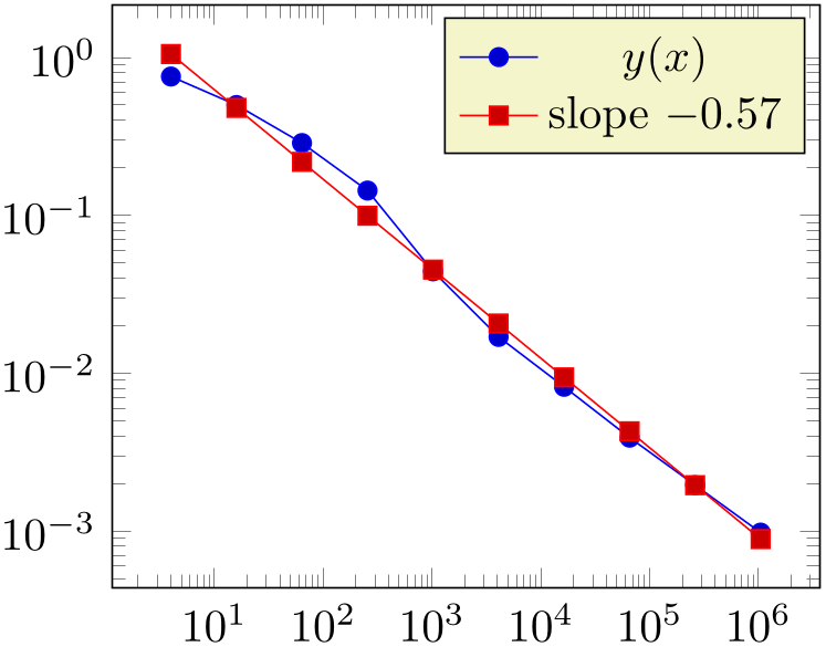
The (commented) line containing \slope is explained above; it allows to remember different regression slopes in our example.
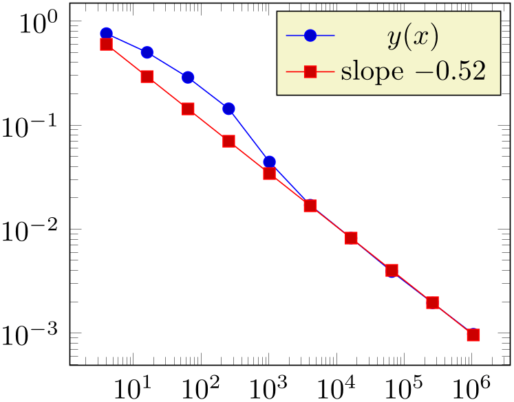
Both keys allow to provide uncertainties (variances) to single data points. A high (relative) variance indicates an unreliable data point, a value of \(1\) is standard.
The variance list key allows to provide variances directly as comma-separated list, for example
variance list={1000,1000,500,200,1,1}.
The
variance key
allows to load values from a table
 column name
 . Such a column name is (initially, see below) loaded from the same table where data points have been found. The
 column name
 may also be a create on use name.

% Preamble: \pgfplotsset{width=7cm,compat=1.18}
\begin{tikzpicture}
\begin{loglogaxis}
                         \addplot table
                        [x=dof,y=error2]
{pgfplotstable.example1.dat};
\addlegendentry{$y(x)$}
                         \addplot table
                        [
x=dof,
                                y={create
                        col/linear regression={
y=error2,
                                    variance
                        list={1000,800,600,500,400},
}}
] {pgfplotstable.example1.dat};
\addlegendentry{slope
$\pgfmathprintnumber{\pgfplotstableregressiona}$}
\end{loglogaxis}
\end{tikzpicture}
If both, variance list and variance are given, the first one will be preferred. Note that it is not necessary to provide variances for every data point.
Allows to load the variance from another table. The initial setting is empty. It is acceptable if the variance column in the external table has fewer entries than expected, in this case, only the first ones will be used.
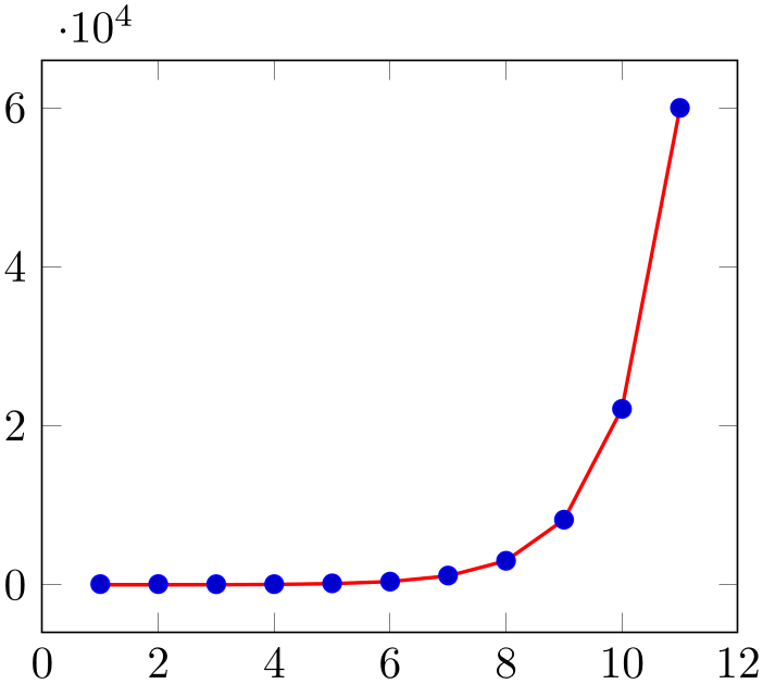
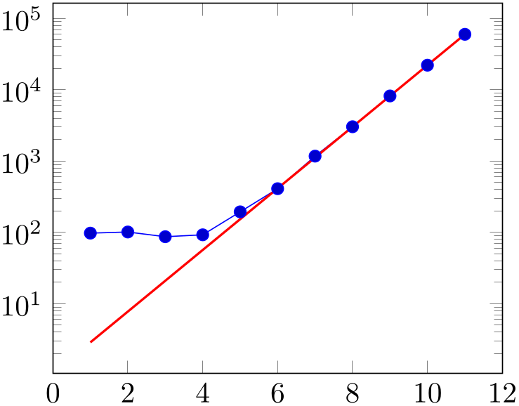
The default configuration assumes that variance is already given in logarithmic coordinates and might prove to be unsuitable for exponential functions. Use variance format=linear in order to map the variance to log coordinates explicitly. This applies even if no variance is specified:
% file plotdata/approx_exp.dat
n eapprox
1 97.71828182845904
2 101.38905609893065
3 87.08553692318768
4 92.59815003314424
5 194.4131591025766
6 410.4287934927351
7 1174.6331584284585
8 3032.9579870417283
9 8198.083927575384
10 22124.465794806718
11 59973.14171519782

% Preamble: \pgfplotsset{width=7cm,compat=1.18}
\begin{tikzpicture}
\begin{axis}
\addplot table[x=n,y=eapprox]
{plotdata/approx_exp.dat};
\addplot[no markers,red,thick]
table [x=n,y={create col/linear regression={
y=eapprox,ymode=log,
variance format=linear}}]
{plotdata/approx_exp.dat};
\end{axis}
\end{tikzpicture}
The option can be specified to the axis environment as well:

% Preamble: \pgfplotsset{width=7cm,compat=1.18}
\begin{tikzpicture}
\begin{axis}[
ymode=log,
table/create col/linear regression/variance format=linear
]
\addplot table[x=n,y=eapprox]
{plotdata/approx_exp.dat};
\addplot[no markers,red,thick]
table [x=n,y={create col/linear regression={
y=eapprox,ymode=log}}]
{plotdata/approx_exp.dat};
\end{axis}
\end{tikzpicture}
Currently, pgfplots supports only linear regression, and it only supports regression together with \addplot table. Furthermore, long input tables might need quite some time.
73 The y={create col/ feature is available for any other PgfplotsTable postprocessing style, see the create on use documentation in the PgfplotsTable manual.
74 In fact, pgfplots sees that there are only two columns and uses the second by default. But you need to provide it if there are at least 3 columns.