Manual for Package pgfplots
2D/3D Plots in LATeX, Version 1.18.2
https://github.com/pgf-tikz/pgfplots
The Reference
4.113D Axis Configuration
This section described keys which are used to configure the appearance of three dimensional figures. Some of them apply for two-dimensional plots as special case as well, and they will also be discussed in the respective sections of this manual.
4.11.1View Configuration
-
/pgfplots/view={
 azimuth
 }{
}{ elevation
 } (initially {25}{30})
Changes both view angles of a 3D axis. The azimuth (first argument) is the horizontal angle which is rotated around the \(z\)-axis. For a 3D plot, the \(z\)-axis always points to the top. The elevation (second argument) is the vertical rotation around the (rotated) \(x\)-axis. Positive elevation values indicate a view from above, negative a view from below. All values are measured in degree (but see trig format).
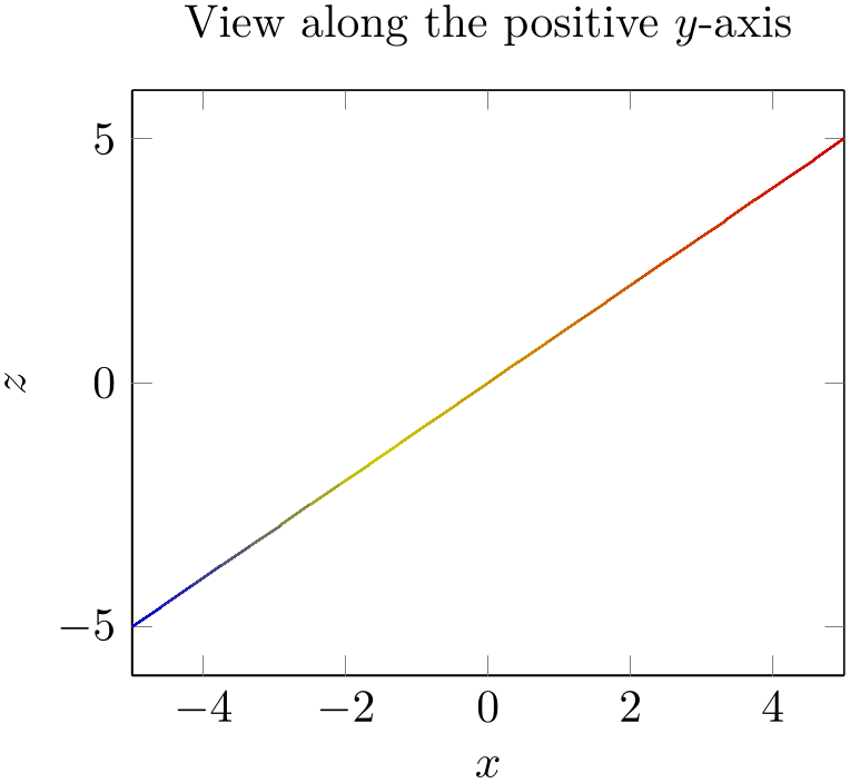
% Preamble: \pgfplotsset{width=7cm,compat=1.18}
\begin{tikzpicture}
\begin{axis}[
view={0}{0},
xlabel=$x$,
zlabel=$z$,
                        title=View along the positive
                    $y$-axis,
]
\addplot3 [surf] {x};
\end{axis}
\end{tikzpicture}
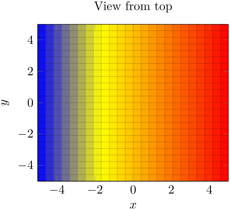
% Preamble: \pgfplotsset{width=7cm,compat=1.18}
\begin{tikzpicture}
\begin{axis}[
view={0}{90},
xlabel=$x$,
ylabel=$y$,
title=View from top,
]
\addplot3 [surf] {x};
\end{axis}
\end{tikzpicture}
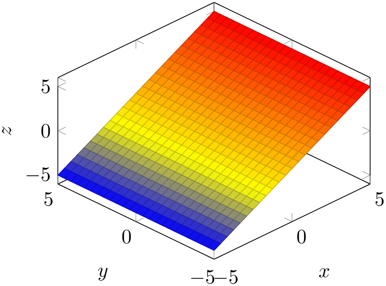
% Preamble: \pgfplotsset{width=7cm,compat=1.18}
\begin{tikzpicture}
\begin{axis}[
view={-45}{45},
xlabel=$x$,
ylabel=$y$,
zlabel=$z$,
]
\addplot3 [surf] {x};
\end{axis}
\end{tikzpicture}
The view is computed as follows. The view is defined
by two rotations: the first rotation uses the
 azimuth
 angle to rotate around the \(z\) axis. Afterwards, the view is rotated
 elevation
 degrees around the rotated \(x\)-axis (more precisely, it is rotated \(-\)
 elevation
 degrees). The resulting transformed \(xz\)-plane is the viewport, i.e. the view direction is always the transformed positive
\(y\)-axis.
The view argument is compatible with the argument of the Matlab® view command, i.e. you can use
[h,v] = view
in Matlab and pack the resulting arguments into pgfplots.58
If you work with gnuplot, you can convert the view arguments as follows: the gnuplot command
set view v,h
is equivalent to view={h}{90-v}. For example, the default gnuplot configuration set view 60,60 is equivalent to view={60}{30} in pgfplots.
The view is (currently) always an orthogonal projection, no perspective is possible, yet. You can, however, specify projection unit vectors for x, y, and z explicitly to get a skewed three-dimensional axis.
-
/pgfplots/view/az={
 azimuth
 }
}
-
/pgfplots/view/h={
 azimuth
 } (initially 25)
Changes only the azimuth view angle, i.e. the horizontal (first) view angle which is rotated around the \(z\)-axis.

% Preamble: \pgfplotsset{width=7cm,compat=1.18}
\begin{tikzpicture}
\begin{axis}[view/h=-30]
\addplot3 [
surf,
% shader=interp,
shader=flat,
samples=50,
domain=-3:3,y domain=-2:2,
]
{sin(deg(x+y^2))};
\end{axis}
\end{tikzpicture}

% Preamble: \pgfplotsset{width=7cm,compat=1.18}
\begin{tikzpicture}
\begin{axis}[view/h=10]
\addplot3 [
surf,
% shader=interp,
shader=flat,
samples=50,
domain=-3:3,y domain=-2:2,
]
{sin(deg(x+y^2))};
\end{axis}
\end{tikzpicture}

% Preamble: \pgfplotsset{width=7cm,compat=1.18}
\begin{tikzpicture}
\begin{axis}[view/h=40,colormap/violet]
\addplot3 [
surf,
% shader=interp,
shader=flat,
samples=50,
domain=-3:3,y domain=-2:2,
]
{sin(deg(x+y^2))};
\end{axis}
\end{tikzpicture}
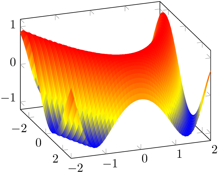
% Preamble: \pgfplotsset{width=7cm,compat=1.18}
\begin{tikzpicture}
\begin{axis}[view/h=70]
\addplot3 [
surf,
% shader=interp,
shader=flat,
samples=50,
domain=-3:3,y domain=-2:2,
]
{sin(deg(x+y^2))};
\end{axis}
\end{tikzpicture}
4.11.2Styles Used Only For 3D Axes
-
/pgfplots/every 3d description(style, no value) 
This style allows to change the appearance of descriptions for three dimensional axes. Naturally, a three dimensional axis will display axis labels for \(x\) and \(y\) differently than a two dimensional axis (for example, the \(y\)-axis label won’t be rotated by 90 degrees). The every 3d description style installs the necessary display options for three dimensional axis descriptions.
The initial value is:
\pgfkeys{
/pgfplots/every 3d description/.style={
% Only these description styles can be changed here:
every axis x label/.style={
at={(ticklabel cs:0.5)},
anchor=near ticklabel,
},
every axis y label/.style={
at={(ticklabel cs:0.5)},
anchor=near ticklabel,
},
every x tick scale label/.style={
at={(xticklabel cs:0.95,5pt)},
anchor=near xticklabel,
inner sep=0pt,
},
every y tick scale label/.style={
at={(yticklabel cs:0.95,5pt)},
anchor=near yticklabel,
inner sep=0pt,
},
try min ticks=3,
},
}
As the name suggests, every 3d description can only be used to set styles for axis labels, tick labels and titles. It has not been designed to reset other styles, you will need to change these options either for each axis separately or by means of user defined styles. The reason for this limitation is: other options can (and, in many cases, needs to) be set before the axis is processed. However, the decision whether we have a two dimensional or a three dimensional axis has to be postponed until the processing is more or less complete – so only some remaining keys can be set.
-
/pgfplots/every 3d view {
 h
h }{
}{ v
v }(style, no value)
A style which can be used for fine-tuning of the output for specific views.
This style will be installed right after every 3d description, but before other axis description related keys are set (in other words: it has higher precedence than every 3d description, but lower precedence than keys provided to the axis directly).
One example is pre-configured for view={0}{90} (from top):
\pgfplotsset{
/pgfplots/every 3d view {0}{90}/.style={
xlabel near ticks,
ylabel near ticks,
axis on top=true,
},
}
4.11.3Appearance Of The 3D Box
-
/pgfplots/plot box ratio={

 x stretch
 y stretch
 z stretch
 } (initially 1 1 1)
Allows to customize the aspect ratio between the three different axes in a three dimensional plot.
Note that this key is different from the related unit vector ratio: the plot box is only useful for three dimensional axes, and it will usually distort the unit vector ratios. If you want equal unit ratios, consider using unit vector ratio.
The plot box ratio is applied before any rotations and stretch-to-fill routines have been invoked. Thus, the initial setting59 1 1 1 makes all axes equally long before the stretch-to-fill routine is applied.
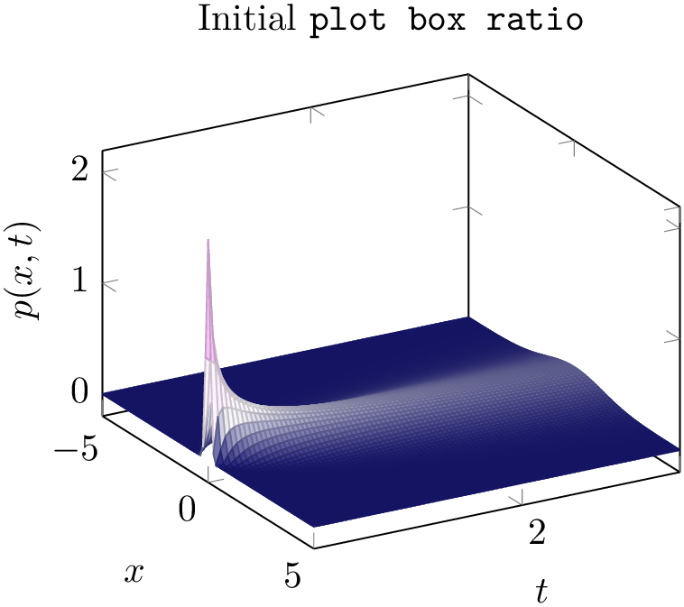
% Preamble: \pgfplotsset{width=7cm,compat=1.18}
\begin{tikzpicture}
\begin{axis}[
view/h=60,
plot box ratio=1 1 1,
colormap={violet}{[1cm] rgb255(0cm)=(25,25,122)
color(1cm)=(white) rgb255(5cm)=(238,140,238)},
xlabel=$x$,
ylabel=$t$,
zlabel={$p(x,t)$},
shader=faceted,
                        title=Initial \texttt{plot box
                    ratio},
]
\addplot3 [surf,y domain=0.02:3.5,samples=81]
{1/(2*sqrt(pi*y)) * exp(0-x^2/y)};
% the '0' is a workaround for a bug in PGF 2.00
\end{axis}
\end{tikzpicture}
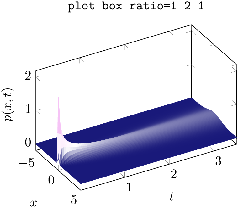
% Preamble: \pgfplotsset{width=7cm,compat=1.18}
\begin{tikzpicture}
\begin{axis}[
view/h=60,
plot box ratio=1 2 1,
colormap={violet}{[1cm] rgb255(0cm)=(25,25,122)
color(1cm)=(white) rgb255(5cm)=(238,140,238)},
xlabel=$x$,
ylabel=$t$,
zlabel={$p(x,t)$},
shader=flat,
                        title=\texttt{plot box ratio=1
                    2 1},
]
\addplot3 [surf,y domain=0.02:3.5,samples=81]
{1/(2*sqrt(pi*y)) * exp(0-x^2/y)};
% the '0' is a workaround for a bug in PGF 2.00
\end{axis}
\end{tikzpicture}
This key applies only to three dimensional axes. After the scaling, the axes will be stretched to fill the width and height for this plot. Thus, the effects of plot box ratio might be undone by this stretching for particular views.
-
/pgfplots/3d box=background|complete|complete* (initially background) 
Allows to configure the appearance of boxed three dimensional axes.
Type only 3d box (without value) as alias for 3d box=complete.
The choice background is the initial setting, it does not draw axis lines (and grid lines) which are in the foreground.

% Preamble: \pgfplotsset{width=7cm,compat=1.18}
\begin{tikzpicture}
\begin{axis}[
3d box=background,
% pretty printing, but irrelevant:
title={3d box=background},
samples=5,
domain=-4:4,
xtick=data,
ytick=data,
]
\addplot3 [surf] {x*y};
\end{axis}
\end{tikzpicture}
The choice complete also draws axis lines and tick lines in the foreground, but it doesn’t draw grid lines in the foreground. The result yields a complete box:
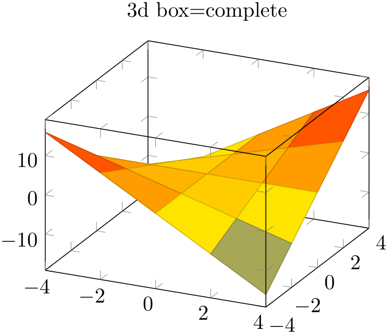
% Preamble: \pgfplotsset{width=7cm,compat=1.18}
\begin{tikzpicture}
\begin{axis}[
                        3d box,% same as 3d
                    box=complete
% pretty printing, but irrelevant:
title={3d box=complete},
samples=5,
domain=-4:4,
xtick=data,
ytick=data,
]
                            \addplot3
                    [surf] {x*y};
\end{axis}
\end{tikzpicture}
Finally, the choice complete* is the same as complete, but it also draws grid lines in the foreground.
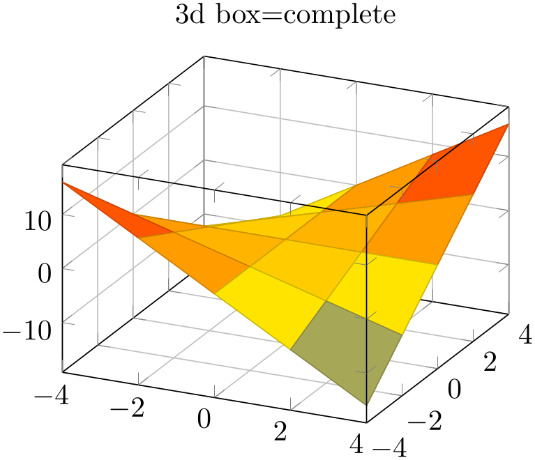
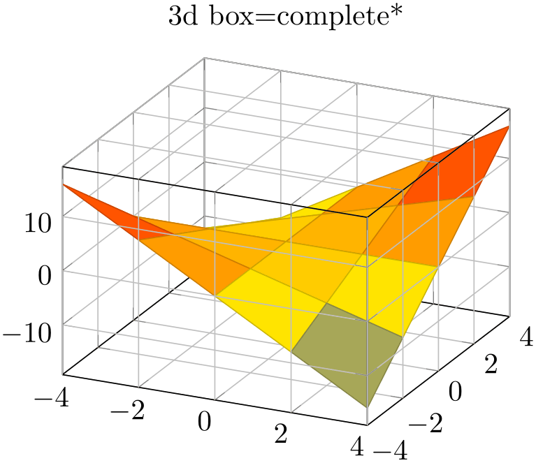
% Preamble: \pgfplotsset{width=7cm,compat=1.18}
\begin{tikzpicture}
\begin{axis}[
3d box=complete,
grid=major,
title={3d box=complete},
samples=5, domain=-4:4,
xtick=data, ytick=data,
]
                            \addplot3
                    [surf] {x*y};
\end{axis}
\end{tikzpicture}%
~
\begin{tikzpicture}
\begin{axis}[
3d box=complete*,
grid=major,
title={3d box=complete*},
samples=5, domain=-4:4,
xtick=data, ytick=data,
]
\addplot3
[surf] {x*y};
\end{axis}
\end{tikzpicture}
Before any foreground parts are actually processed, the style every 3d box foreground will be installed. This allows to change the appearance of foreground axis components like tick style or axis line style separately from the background components.
Note that 3d box=complete is only available for boxed axes, i.e. together with axis lines=box. It is an error to use a different combination.
4.11.4Axis Line Variants
Three dimensional axes also benefit from the axis lines=box or axis lines=center styles discussed in Section 4.9.9. The choice axis lines=box is standard, it draws a box (probably affected by the 3d box=complete key). The choice axis lines=center draws all three axes such that they pass through the origin. It might be necessary to combine this key with axis on top as there is no depth information.
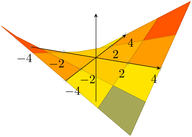
% Preamble: \pgfplotsset{width=7cm,compat=1.18}
% Attention: use compat=1.8 or higher
% to repair label positions
\begin{tikzpicture}
\begin{axis}[
axis lines=center,
axis on top,
samples=5, domain=-4:4,
xtick=data, ytick=data,
ztick=\empty, % no z ticks here
]
\addplot3 [surf] {x*y};
\end{axis}
\end{tikzpicture}
The remaining choices axis lines*=left and axis lines*=right select different sets of axes in a way such that tick labels and axis label won’t disturb the plot’s content. The ‘*’ suppresses the use of special styles which are mainly adequate for two-dimensional axes, see the documentation of axis lines. Such a set of axes is always on the boundary of the two-dimensional projection.
The choice axis lines*=left chooses a set of axes which are on the left (or bottom, respectively) whereas the choice axis lines*=right chooses a set of axes which are on the right (or top, respectively):
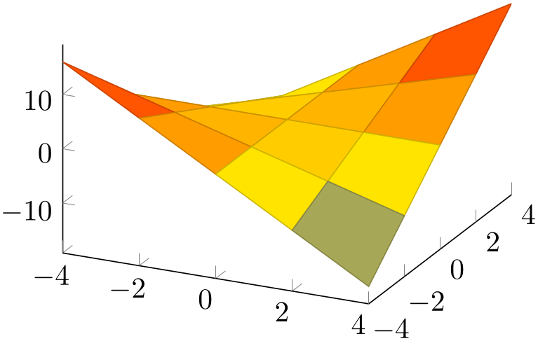
% Preamble: \pgfplotsset{width=7cm,compat=1.18}
\begin{tikzpicture}
\begin{axis}[
axis lines*=left,
samples=5, domain=-4:4,
xtick=data, ytick=data,
]
\addplot3 [surf] {x*y};
\end{axis}
\end{tikzpicture}

% Preamble: \pgfplotsset{width=7cm,compat=1.18}
\begin{tikzpicture}
\begin{axis}[
axis lines*=right,
samples=5, domain=-4:4,
xtick=data, ytick=data,
]
\addplot3 [surf] {x*y};
\end{axis}
\end{tikzpicture}
It is not possible to mix different styles like axis x line=center,axis z line=top.