Manual for Package pgfplots
2D/3D Plots in LATeX, Version 1.18.1
http://sourceforge.net/projects/pgfplots

\usepgfplotslibrary{fillbetween} % LaTeX and plain TeX ¶

\usepgfplotslibrary[fillbetween] % ConTeXt ¶

\usetikzlibrary{pgfplots.fillbetween} % LaTeX and plain TeX ¶

\usetikzlibrary[pgfplots.fillbetween] % ConTeXt ¶

The fillbetween library allows to fill the area between two arbitrary named plots. It can also identify segments of the intersections and fill the segments individually.

\addplot fill between [{options defined with prefix /tikz/fill between}] ; ¶

\addplot[options] fill between [{options defined with prefix /tikz/fill between}] trailing path commands; ¶

\addplot3 … ¶

A special plotting operation which takes two named paths on input and generates one or more paths resembling the filled area between the input paths.



copy % Preamble: \pgfplotsset{width=7cm,compat=1.18}\usepgfplotslibrary{fillbetween} \begin{tikzpicture} \begin{axis} \addplot+ [name path=A,domain=0:1,samples=2] {x}; \addplot+ [name path=B] table { x y 0 2 0.5 -1 1 3 }; \addplot fill between [of=A and B]; \end{axis} \end{tikzpicture}

The operation fill between requires at least one input key within options defined with prefix /tikz/fill between: the two involved paths in the form of=first and second. Here, both first and second need to be defined using name path (or name path global). The arguments can be exchanged,⁸⁶ i.e. we would achieve the same effect for of=B and A.

The argument options defined with prefix /tikz/fill between can contain any number of options which have the prefix /tikz/fill between. Note that the prefix refers to the reference manual, you do not need to type the prefix. This excludes drawing options like fill=orange; these options should be given as options (or inside of styles like every segment). Allowed options include of, split, soft clip, and style definitions of every segment and its friends, i.e. those which define which paths are to be acquired and how they should be processed before they can be visualized.

A fill between operation takes the two input paths, analyzes their orientation (i.e. are its coordinates given increasing in \(x\) direction?), connects them, and generates a fill path.

As mentioned above, the input paths need to be defined in advance (forward references are unsupported). If you would generate the filled path manually, you would draw it before the other ones such that it does not overlap. This is done implicitly by pgfplots: as soon as pgfplots encounters a fill between plot, it will activate layered graphics. The filled path will be placed on layer pre main which is between the main layer and the background layer.

A fill between operation is just like a usual plot: it makes use of the cycle list, i.e. it receives default plot styles. Our first example above uses the default cycle list which has a brown color. We can easily redefine the appearance just as for any other plot by adding options in square braces:



copy % Preamble: \pgfplotsset{width=7cm,compat=1.18}\usepgfplotslibrary{fillbetween} \begin{tikzpicture} \begin{axis} \addplot [blue,name path=A,domain=0:1] {sqrt(x)}; \addplot [red, name path=B,domain=0:1] {sqrt(x/2)}; \addplot [gray] fill between [of=A and B]; \end{axis} \end{tikzpicture}

Note that the number of data points does not restrict fill between. In particular, you can combine different arguments easily.



copy % Preamble: \pgfplotsset{width=7cm,compat=1.18}\usepgfplotslibrary{fillbetween} \begin{tikzpicture} \begin{axis} \addplot [blue,name path=A,domain=0:1] {sin(360*x)}; \addplot [red, name path=B,domain=0:1,samples=2] {0.5}; \addplot [orange] fill between [of=A and B]; \end{axis} \end{tikzpicture}

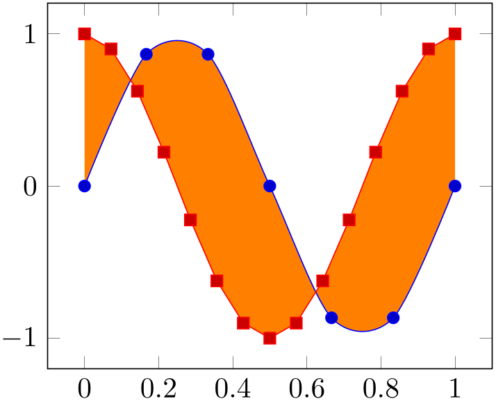
The combination of input plots is also possible if one or both of the plots make use of smooth interpolation:



copy % Preamble: \pgfplotsset{width=7cm,compat=1.18}\usepgfplotslibrary{fillbetween} \begin{tikzpicture} \begin{axis} \addplot+ [name path=A,samples=7,smooth,domain=0:1] {sin(360*x)}; \addplot+ [name path=B,samples=15,domain=0:1] {cos(360*x)}; \addplot [orange] fill between [of=A and B]; \end{axis} \end{tikzpicture}

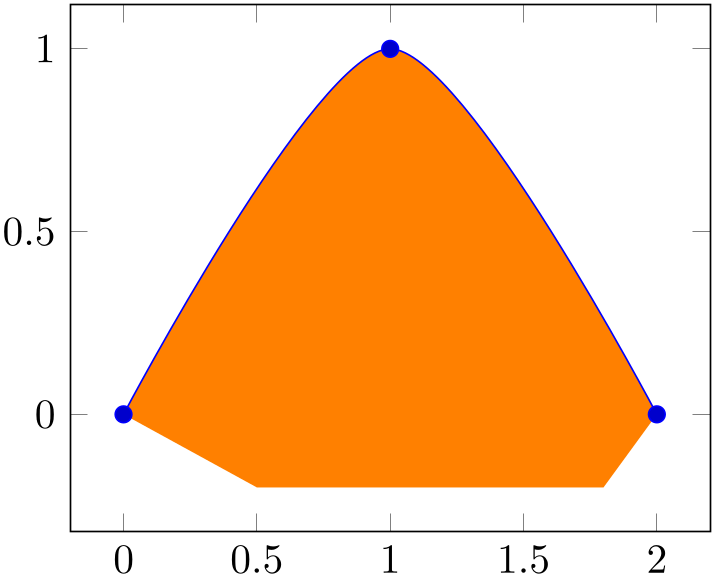
Actually, a fill between path operates directly on the low-level input path segments. As such, it is much closer to, say, a TikZ decoration than to a plot; only its use cases (legends, styles, layering) are tailored to the use as a plot. However, the input paths can be paths and/or plots. The example below combines one \addplot and one \path.



copy % Preamble: \pgfplotsset{width=7cm,compat=1.18}\usepgfplotslibrary{fillbetween} \begin{tikzpicture} \begin{axis}[ymin=-0.2,enlargelimits] \addplot+ [name path=A,smooth] coordinates {(0,0) (1,1) (2,0)}; \path [name path=B] (0.5,-0.2) -- (1.8,-0.2); \addplot [orange] fill between [of=A and B]; \end{axis} \end{tikzpicture}

As mentioned above, fill between takes the two input paths as such and combines them to a filled segment. To this end, it connects the endpoints of both paths. This can be seen in the example above: the path named ‘B’ has different \(x\)-coordinates than ‘A’ and results in a trapezoidal output.

Here is another example in which a plot and a normal path are combined using fill between. Note that the \draw path is generated using nodes of path ‘A’. In such a scenario, we may want to fill only the second segment which is also possible, see split below.



copy % Preamble: \pgfplotsset{width=7cm,compat=1.18}\usepgfplotslibrary{fillbetween} \begin{tikzpicture} \begin{axis} \addplot+ [name path=A,samples=15,domain=0:1] {cos(360*x)} coordinate [pos=0.25] (nodeA0) {} coordinate [pos=0.75] (nodeA1) {}; \draw [name path=B] (nodeA0) -- (nodeA1); \addplot [orange] fill between [of=A and B]; \end{axis} \end{tikzpicture}

A fill between plot is different from other plotting operations with respect to the following items:

• 1. It has no own markers and no nodes near coords. However, its input paths can have both.

• 2. It supports no pos nodes. However, its input paths can have any annotations as usual.

• 3. It supports no error bars. Again, its input paths support what pgfplots offers for plots.

• 4. It cannot be stacked (its input plots can be, of course).

Note that more examples can also be found in Section 4.5.10.2 on page (page for section 4.5.10.2) which covers Area Plots and has a lot of examples on fill between.

/tikz/fill between/split=true|false (initially false) ¶

Activates the generation of more than one output segment.

The initial choice split=false is quite fast and robust, it simply concatenates the input paths and generates exactly one output segment.

The choice split=true results in a computation of every intersection of the two curves (by means of the tikz library intersections). Then, each resulting segment results in a separate drawing instruction.

The choice split=false is the default and has been illustrated with various examples above.

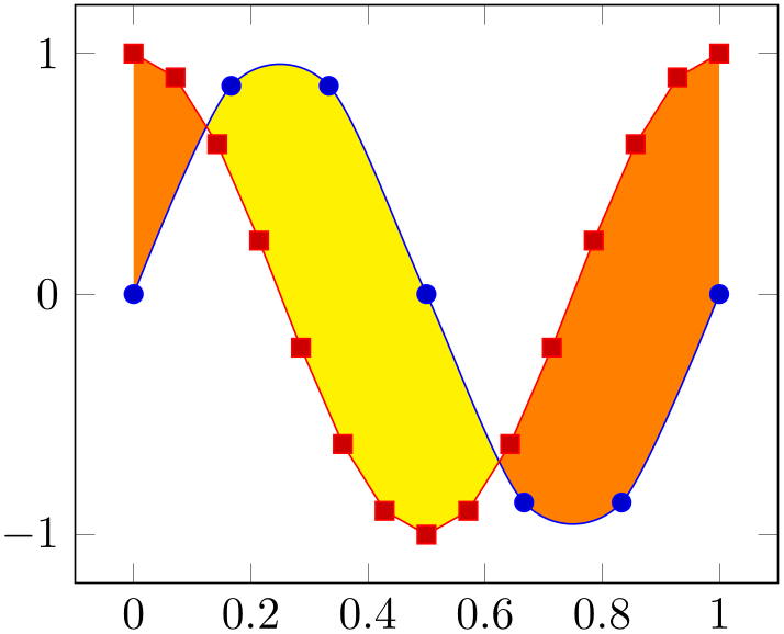
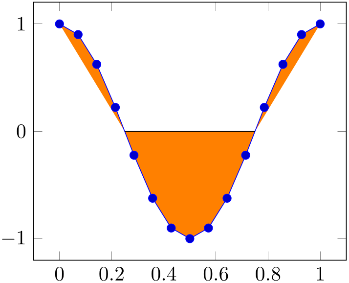
The choice split=true is very useful in conjunction with the various styles. For example, we could use every odd segment to choose a different color for every odd segment:



copy % Preamble: \pgfplotsset{width=7cm,compat=1.18}\usepgfplotslibrary{fillbetween} \begin{tikzpicture} \begin{axis} \addplot+ [name path=A,samples=7,smooth,domain=0:1] {sin(360*x)}; \addplot+ [name path=B,samples=15,domain=0:1] {cos(360*x)}; \addplot [orange] fill between [of=A and B, split, every odd segment/.style={yellow}, ]; \end{axis} \end{tikzpicture}

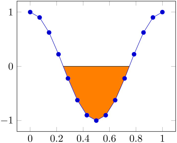
Similarly, we could style the regions individually using every segment no:



copy % Preamble: \pgfplotsset{width=7cm,compat=1.18}\usepgfplotslibrary{fillbetween} \begin{tikzpicture} \begin{axis} \addplot+ [name path=A,samples=15, smooth,domain=0:1] {sin(720*x)}; \path [name path=B] (\pgfkeysvalueof{/pgfplots/xmin},0) -- (\pgfkeysvalueof{/pgfplots/xmax},0) ; \addplot fill between [of=A and B, split, every segment no 0/.style= {orange}, every segment no 1/.style= {pattern=north east lines}, every segment no 2/.style= {pattern=north west lines}, every segment no 3/.style= {top color=orange, bottom color=blue}, ]; \end{axis} \end{tikzpicture}

The split option allows us to revisit our earlier example in which we wanted to draw only one of the segments:



copy % Preamble: \pgfplotsset{width=7cm,compat=1.18}\usepgfplotslibrary{fillbetween} \begin{tikzpicture} \begin{axis} \addplot+ [name path=A,samples=15,domain=0:1] {cos(360*x)} coordinate[pos=0.25] (nodeA0) coordinate[pos=0.75] (nodeA1) ; \draw [name path=B] (nodeA0) -- (nodeA1); \addplot [fill=none] % default: fill none fill between [of=A and B, split, % draw only selected ones: % every segment no 0/.style: invisible every segment no 1/.style={fill,orange}, % every segment no 2/.style: invisible ]; \end{axis} \end{tikzpicture}

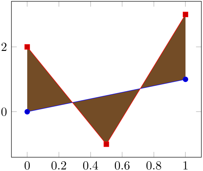
Each segment results in an individual \fill instruction, i.e. each segment is its own, independent, path. This allows to use all possible TikZ path operations, including pattern, shade, or decorate.



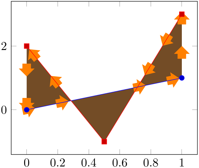
copy % Preamble: \pgfplotsset{width=7cm,compat=1.18}\usepgfplotslibrary{fillbetween} % requires % \usetikzlibrary{decorations.markings,shapes.arrows} \begin{tikzpicture} \begin{axis} \addplot+ [name path=A,domain=0:1,samples=2] {x}; \addplot+ [name path=B] table { x y 0 2 0.5 -1 1 3 }; \addplot fill between [of=A and B, split, every even segment/.style={ postaction={decorate}, decoration={ markings, mark=between positions 0 and 1 step 1cm with { \node [single arrow,fill=orange, single arrow head extend=3pt, transform shape] {}; }, }, }, ]; \end{axis} \end{tikzpicture}

/tikz/fill between/soft clip=argument ¶

/tikz/fill between/soft clip first=argument ¶

/tikz/fill between/soft clip second=argument ¶

Installs “soft-clips” on both or just one of the involved paths. Soft-clipping means to modify the input paths such that they respect a clipping region.

In its default configuration, fill between connects the start/end points of the two involved paths.

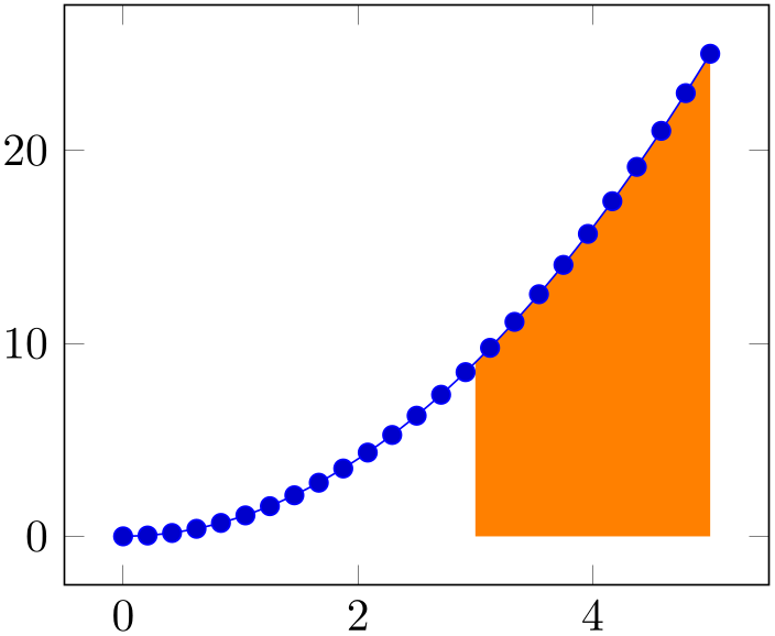
This is often what you want, but there are use cases where only parts between the input parts should be filled: suppose we have \(f(x)=x^2\) and we want to fill below the interval \([3,5]\). The case “fill below” means to fill between our function and the \(x\)-axis:



copy % Preamble: \pgfplotsset{width=7cm,compat=1.18}\usepgfplotslibrary{fillbetween} \begin{tikzpicture} \begin{axis} \addplot+ [name path=A,domain=0:5] {x^2}; \path [name path=B] (\pgfkeysvalueof{/pgfplots/xmin},0) -- (\pgfkeysvalueof{/pgfplots/xmax},0); \addplot [orange] fill between [of=A and B]; \end{axis} \end{tikzpicture}

Clearly, we have filled too much. A solution might be to shorten the path B – but that would still connect the left and right end points of \(f(x)\) with the shortened line.

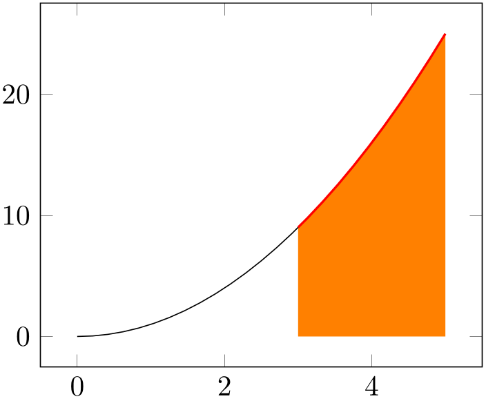
This is where soft clip has its uses: we can select the area of interest by installing a soft clip path:



copy % Preamble: \pgfplotsset{width=7cm,compat=1.18}\usepgfplotslibrary{fillbetween} \begin{tikzpicture} \begin{axis} \addplot+ [name path=A,domain=0:5] {x^2}; \path [name path=B] (\pgfkeysvalueof{/pgfplots/xmin},0) -- (\pgfkeysvalueof{/pgfplots/xmax},0); \addplot [orange] fill between [ of=A and B, soft clip={domain=3:5}, ]; \end{axis} \end{tikzpicture}

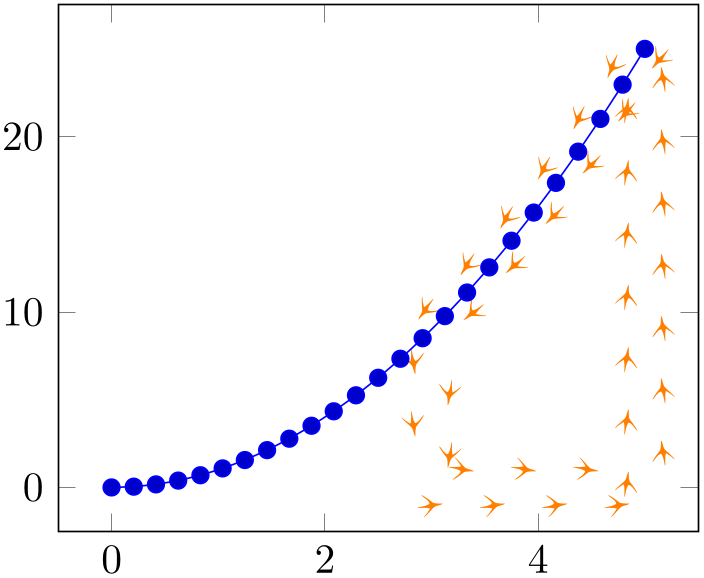
Soft-clipping is similar to clipping. In fact, we could have installed a clip path to achieve the same effect.⁸⁷ However, soft-clipping results in a new path which is aware of the boundaries. Consequently, decorations will be correct, without suffering from missing image parts due to the clipping:



copy % Preamble: \pgfplotsset{width=7cm,compat=1.18}\usepgfplotslibrary{fillbetween} \begin{tikzpicture} \begin{axis} \addplot+ [name path=A,domain=0:5] {x^2}; \path [name path=B] (\pgfkeysvalueof{/pgfplots/xmin},0) -- (\pgfkeysvalueof{/pgfplots/xmax},0); \addplot[ orange, decorate,decoration={ footprints, foot of=bird, stride length=15pt, foot sep=2pt, foot length=6pt, }, ] fill between [ of=A and B, soft clip={domain=3:5}, ]; \end{axis} \end{tikzpicture}

The feature soft clip is a part of fill between in the sense that it determines the fill path.

The argument can be one of the following items:

• • It can be of the form domain=xmin:xmax. This choice is equivalent to

  (xmin,\pgfkeysvalueof{/pgfplots/ymin}) rectangle

  (xmax,\pgfkeysvalueof{/pgfplots/ymax}).

• • It can be of the form domain y=ymin:ymax. This choice is equivalent to

  (\pgfkeysvalueof{/pgfplots/xmin},ymin) rectangle

  (\pgfkeysvalueof{/pgfplots/xmax},ymax).

• • It can be (x,y) rectangle (X,Y ). In this case, it is the rectangle defined by the given points.

• • It can be the name of a named path, i.e. soft clip=A if there exists a path with name path=A.

  In this case, the named path has to be “reasonable simple”. In particular, it should be convex, that is like a rectangle, a circle, or some cloud. It should also be closed.

In any case, the soft clip path should be larger than the paths it applies to. Please avoid infinitely many intersections points.



copy % Preamble: \pgfplotsset{width=7cm,compat=1.18}\usepgfplotslibrary{fillbetween} \begin{tikzpicture} \begin{axis} \draw [help lines,name path=clippath] (0,-5) -- (-5,0) -- (2,4) -- (4,-4) --cycle; \addplot+ [name path=A] {x}; \draw [red,name path=B] (0,\pgfkeysvalueof{/pgfplots/ymin}) -- (0,\pgfkeysvalueof{/pgfplots/ymax}); \addplot[gray!50] fill between [ of=A and B, soft clip={clippath} ]; \end{axis} \end{tikzpicture}

The previous example defines three named paths: the path A is \(f(x) = x\). The named path clippath serves as clip path, it is some rotated rectangular form. Finally, the path named B is a straight line – and we fill between A and B with the given clippath.

The choice soft clip first applies the clip path only to the first input path (“A” in our case).

The choice soft clip second applies the clip path only to the second input path (“B” in our case).

Finally, soft clip applies the clip path to both input paths.



copy % Preamble: \pgfplotsset{width=7cm,compat=1.18}\usepgfplotslibrary{fillbetween} % requires \usepgfplotslibrary{fillbetween} \begin{tikzpicture} \begin{axis} \addplot+ [name path=A,domain=0:5] {x^2}; \path [name path=B] (\pgfkeysvalueof{/pgfplots/xmin},0) -- (\pgfkeysvalueof{/pgfplots/xmax},0); \addplot [gray] fill between [ of=A and B, soft clip={ (3,-1) rectangle (4,100) }, ]; \addplot [gray!30] fill between [ of=A and B, soft clip={ (2,-1) rectangle (3,100) }, ]; \end{axis} \end{tikzpicture}

Note that there is also a separate module which allows to apply soft-clipping to individual paths. To this end, a decoration=soft clip is available. A use case could be to highlight parts of the input path:



copy % Preamble: \pgfplotsset{width=7cm,compat=1.18}\usepgfplotslibrary{fillbetween} \begin{tikzpicture} \begin{axis} \addplot [name path=A,domain=0:5, postaction={decorate,red,thick}, decoration={ soft clip, soft clip path={domain=3:5}, }, ] {x^2}; \path [name path=B] (\pgfkeysvalueof{/pgfplots/xmin},0) -- (\pgfkeysvalueof{/pgfplots/xmax},0); \addplot [orange] fill between [ of=A and B, soft clip={ (3,-1) rectangle (5,100) }, ]; \end{axis} \end{tikzpicture}

Note that more examples can also be found in Section 4.5.10.2 on page (page for section 4.5.10.2) which covers Area Plots and has a lot of examples on fill between.

/tikz/fill between/every segment(style, no value) ¶

A style which installed for every segment generated by fill between.

The sequence of styles which are being installed is

every segment, any options provided after \addplot[options] fill between, then the appropriate every segment no index, then one of every odd segment or every even segment, then every last segment.

/tikz/fill between/every odd segment(style, no value) ¶

A style which is installed for every odd segment generated by fill between.

Attention: this style makes only sense if split is active.

See every segment for the sequence in which the styles will be invoked.

/tikz/fill between/every even segment(style, no value) ¶

A style which is installed for every even segment generated by fill between.

Attention: this style makes only sense if split is active.

See every segment for the sequence in which the styles will be invoked.

/tikz/fill between/every segment no index(style, no value) ¶

A style which is installed for every segment with the designated index index generated by fill between.

An index is a number starting with \(0\) (which is used for the first segment).

Attention: this style makes only sense if split is active.

See every segment for the sequence in which the styles will be invoked.

/tikz/fill between/every last segment(style, no value) ¶

A style which installed for every last segment generated by fill between.

\tikzsegmentindex ¶

A command which is valid while the paths of \addplot fill between are generated.

It expands to the segment index, i.e. the same value which is used by every segment no index.

An index is a number starting with \(0\) (which is used for the first segment).

/pgfplots/every fill between plot(style, no value) ¶

A style which is installed for every \addplot fill between. Its default is

copy \pgfkeys{ /pgfplots/every fill between plot/.style={ /pgfplots/area legend,/tikz/fill}, }

/tikz/fill between/of=first and second ¶

This key is mandatory. It defines which paths should be combined.

The arguments are names which have been assigned to paths or plots in advance using name path. Paths with these two names are expected in the same tikzpicture.

The fillbetween library supports a variety of input paths, namely

• • plots of functions, i.e. each \(x\)-coordinate has at most one \(y\)-coordinate,

• • plots with interruptions,

• • TikZ paths which meet the same restrictions and are labelled by name path,

• • smooth curves or curveto paths,

• • mixed smooth non-smooth parts.

However, it has at most restricted support (or none at all) for paths which

• • have self-intersections (i.e. parametric plots might pose a problem),

• • have coordinates which are given in a strange input sequence,

• • consist of lots of individually separated sub-paths (like mesh or surf plots).

Note that the input paths do not necessarily need to be given in the same sequence, see fill between/reverse.

/tikz/name path={name} ¶

A TikZ instruction which assigns a name to a path or plot.⁸⁸

This is mandatory to define input arguments for fill between/of.

/tikz/fill between/reverse=auto|true|false (initially auto) ¶

Configures whether the input paths specified by of need to be reversed in order to arrive at a suitable path concatenation.

The initial choice auto will handle this automatically. To this end, it applies the following heuristics: it compares the two first coordinates of each plot: if both plots have their \(x\)-coordinates in ascending order, one of them will be reversed (same if both are in descending order). If one is in ascending and on in descending, they will not be reversed. If the \(x\)-coordinates of the first two points are equal, the \(y\)-coordinates are being compared.

The choice true will always reverse one of the involved paths. This is suitable if both paths have the same direction (for example, both are specified in increasing \(x\) order).

The choice false will not reverse the involved paths. This is suitable if one path has, for example, coordinates in increasing \(x\) order whereas the other path has coordinates in decreasing \(x\) order.

Manual reversal is necessary if pgfplots chose the wrong one.



copy % Preamble: \pgfplotsset{width=7cm,compat=1.18}\usepgfplotslibrary{fillbetween} \begin{tikzpicture} \begin{axis} \addplot [blue,-stealth,name path=A] {x}; \draw [-stealth,name path=B] (0,-5) -- (0,5); \addplot [gray!50] fill between [of=A and B,reverse=true]; \end{axis} \end{tikzpicture}

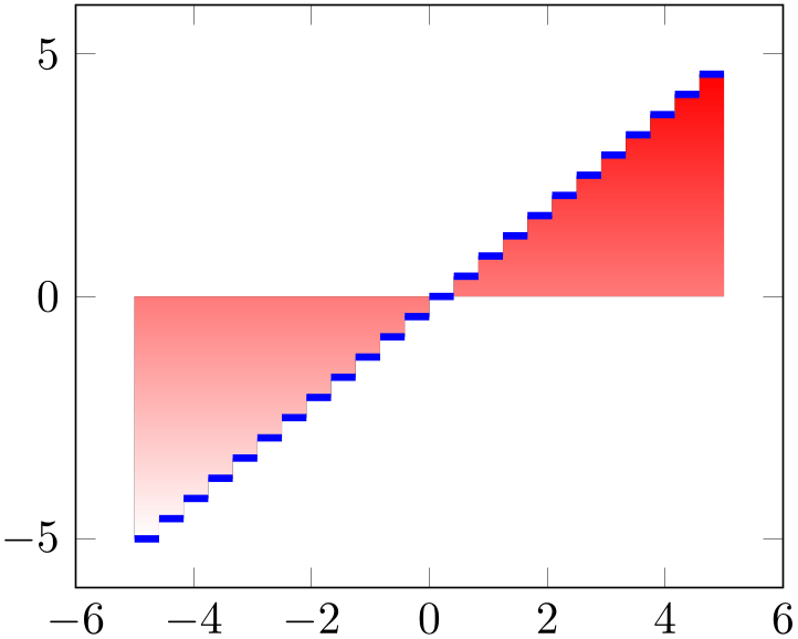
In this case, we chose reverse=true. This is essentially equivalent to the instruction

• • use path A

• • append the reversed path B

• • fill the result.

In other words, it is equivalent to the following path construction based on intersection segments:



copy % Preamble: \pgfplotsset{width=7cm,compat=1.18}\usepgfplotslibrary{fillbetween} \begin{tikzpicture} \begin{axis}[set layers] \addplot [blue,-stealth,name path=A] {x}; \draw [-stealth,name path=B] (0,-5) -- (0,5); \pgfonlayer{pre main} \fill [ gray!50, intersection segments={ of=A and B, sequence={A* -- B*[reverse]}, }, ]; \endpgfonlayer \end{axis} \end{tikzpicture}

Here, we filled the intersection segments of A and B by taking all (indicated by *) segments of A and all of B in reversed order.



copy % Preamble: \pgfplotsset{width=7cm,compat=1.18}\usepgfplotslibrary{fillbetween} \begin{tikzpicture} \begin{axis} \addplot [blue,-stealth,name path=A] {x}; \draw [-stealth,name path=B] (0,-5) -- (0,5); \addplot [gray!50] fill between [ of=A and B, reverse=false, ]; \end{axis} \end{tikzpicture}

In this case, we chose reverse=false. This, in turn, can be expressed as

• • use path A,

• • connect with path B,

• • fill the result.

In other words, it resembles the following intersection segments construction:



copy % Preamble: \pgfplotsset{width=7cm,compat=1.18}\usepgfplotslibrary{fillbetween} \begin{tikzpicture} \begin{axis}[set layers] \addplot [blue,-stealth,name path=A] {x}; \draw [-stealth,name path=B] (0,-5) -- (0,5); \pgfonlayer{pre main} \fill [ gray!50, intersection segments={ of=A and B, sequence={A* -- B*}, }, ]; \endpgfonlayer \end{axis} \end{tikzpicture}

/tikz/fill between/on layer={layer name} (initially pre main) ¶

Defines the layer on which \addplot fill between will be drawn. pgfplots defines the layer pre main to be right before the main layer and pre main is also the initial configuration for any fill between path.

As soon as you type \addplot fill between, pgfplots will activate layered graphics using set layers such that this works automatically. pgfplots will also install a clip path the first time it encounters this layer.

Set layer name to the empty string to place deactivate special layer support for fill between.

Note that this auto-activation of set layers and the installation of a clip path is done for \addplot fill between, not for the lower level drawing instructions like \tikzfillbetween or intersection segments. If you need them, you have to install a layer list manually using either set layers (if inside of an axis) or \pgfsetlayers. The clip path for an axis can be installed manually using

copy \pgfplotsextra{ \pgfonlayer{pre main} \pgfplotspathaxisoutline \pgfusepath{clip} \endpgfonlayer }

(should this ever be necessary).

/tikz/fill between/inner moveto=connect|keep (initially connect) ¶

Sometimes input paths contain the leading moveto operation and some inner movetos. This key configures how to deal with them.

The initial choice connect replaces them by lineto operations (and connects them).⁸⁹

The choice keep keeps them.

Typically, fill between requires the initial choice connect as it allows to deal with interrupted paths:



copy % Preamble: \pgfplotsset{width=7cm,compat=1.18}\usepgfplotslibrary{fillbetween} \begin{tikzpicture} \begin{axis} \addplot [blue,ultra thick,name path=A, jump mark left] {x}; \path [name path=B] (-5,0) -- (5,0); \addplot [top color=red, bottom color=white] fill between [of=A and B]; \end{axis} \end{tikzpicture}

/tikz/intersection segments={options with prefix /tikz/segments} ¶

Evaluates options and appends intersection segments to the current path.

This key is actually more a command: it acquires the two input paths which are argument of the mandatory of key and it parses the series specification which is argument of sequence. Afterwards, it computes the intersection segments and concatenates them according to series specification. Each resulting segment is appended to the current path as is.

The key intersection segments can occur more than once in the current path. Since the key generates path elements, it is sufficient to terminate the path right after options have been processed (i.e. to add ‘;’ right after the option list).

Note that this method operates on the transformed paths and does not apply coordinate transformations on its own. It is more like a decoration than a standard path command, although it does not have an input path.

There is also a related key name intersections in the intersections library of TikZ which assigns names to all intersections, see the manual of TikZ for details.

/tikz/segments/of={name1} and {name2} ¶

Defines the two input paths.

/tikz/segments/sequence={series specification} (initially L1 -- R2) ¶

Selects the intersection segments and their sequence.

The series specification consists of a sequence of entries of the form Lindex -- Rindex -- Lindex. It is probably best shown before we delve into the details:



copy % Preamble: \pgfplotsset{width=7cm,compat=1.18}\usepgfplotslibrary{fillbetween} \begin{tikzpicture} \begin{axis}[domain=0:10] \addplot [name path=first,blue] {sin(deg(x)) + 2/5*x}; \addplot [name path=second,red,samples=16,smooth] {cos(deg(1.2*x)) + 2/5*x}; \draw [ black,-stealth, decorate,decoration={ saw, post=lineto, post length=10pt, }, intersection segments={ of=first and second, sequence={ L1 -- R2 -- R3 -- R4 -- L4[reverse] }, }, ]; \end{axis} \end{tikzpicture}

The preceding example defines two input plots of different sampling density, one is a sharp plot and one is smooth. Afterwards, it draws a third path with a saw decoration – and that path concatenates intersection segments.

The entry L1 means to take the first intersection segment of the first input path. In this context, the first input path is always called ‘L’, regardless of its actual name. Note that L1 refers to an entire segment (not just a point).

The second item is -- which means to connect the previous segment with the next one. Without this item, it would have moved to the next one, leaving a gap. Note that -- is normally a connection between two points. In this context, it is a connection between two segments.

The third item is R2 which means to use the second intersection segment of the second input path. Again, the second input path is always called ‘B’, regardless of its actual name. The other items are straightforward until we arrive at L4[reverse]: it is possible to append an reversed path segment this way.

The general syntax is to add an (arbitrary) sequence of [--] [L|R] {index}[options] where options is optional. There is one special case: if index is *, the entire path will be used. If all encountered indices are *, the intersection will not be computed at all (in this case, intersection segments degenerates to “path concatenation”). Consequently, the following example is a degenerate case in which we did “path concatenation” rather than intersection concatenation:



copy \pgfdeclarelayer{pre main} \begin{tikzpicture} \pgfsetlayers{pre main,main} \draw [-stealth,thick,name path=A,red] (0,0) -- (1,1); \draw [-stealth,thick,name path=B,blue] (0,-1) -- (1,0); \pgfonlayer{pre main} \fill [ orange, intersection segments={ of=A and B, sequence={L* -- R*[reverse]}, }, ]; \endpgfonlayer \end{tikzpicture}

Note that segment indices start at \(1\). They will be processed by means of pgf’s math parser and may depend on \pgfintersectionsolutions (which is the number of intersections).

Note that there is actually another syntax: you can use A0-based-index for the first input path and B0-based-index for the second input path. These identifiers were introduced in pgfplots 1.10, but have been deprecated in favor of 1-based indices. The old syntax with 0-based indices will still remain available. It is advised to use L and R instead of A and B.

Note that curly braces around {index} can be omitted if the index has just one digit: L1, L2, or L-2 are all valid.

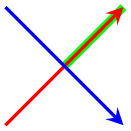
It is also possible to use negative indices to count from the last:



copy \pgfdeclarelayer{pre main} \begin{tikzpicture} \pgfsetlayers{pre main,main} \draw [-stealth,thick,name path=A,red] (0,0) -- (1,1); \draw [-stealth,thick,name path=B,blue] (0,1) -- (1,0); \pgfonlayer{pre main} \draw [ green, line width=2pt, intersection segments={ of=A and B, sequence={L-1}, }, ]; \endpgfonlayer \end{tikzpicture}

In this case \(-1\) denotes the first segment in reverse ordering.

Note that \pgfintersectionsegments is the number of segments in this context.

/tikz/segments/reverse=true|false (false) ¶

Allows to reverse affected path segments.



copy % Preamble: \pgfplotsset{width=7cm,compat=1.18}\usepgfplotslibrary{fillbetween} \begin{tikzpicture} \begin{axis}[xmin=0,xmax=5,ymin=0,ymax=5] \addplot [name path=f,domain=0:5,samples=100] {(x - 2)^2/(7*x) + 1}; \addplot [name path=border, color=blue, ultra thick, dashed] coordinates {(2,0) (2,5) } ; \fill [ intersection segments={ of=f and border, sequence={L1 -- R2}}, pattern=north east lines, ] -- cycle; \fill [ intersection segments={ of=f and border, sequence={R2[reverse] -- L2}}, pattern=north west lines, ] -- (rel axis cs:1,1) -- cycle; \end{axis} \end{tikzpicture}

The preceding example defines two input plots: the plot named f which is the plot of the curve and the blue border line.

It then computes fills paths relying on two intersection segments, one which resembles the part above the curve which is left of the border and one which resembles the part on the right of the border.

It works by concatenating intersection segments in a suitable sequence (add further \draw statements to visualize the individual segments). Note that R2 is used twice: once in normal direction and once reversed. The intersection segments merely constitute the start of the paths; they are extended by --cycle and -- (rel axis cs:1,1) -- cycle, respectively. Keep in mind that rel axis cs is a relative coordinate system in which 1 means \(100\%\) of the respective axis – in this case, we have the upper right corner which is \(100\%\) of \(x\) and \(100\%\) of \(y\).

\tikzfillbetween[options]{draw style} ¶

This is the low-level interface of fill between; it generates one or more paths.

This command can be used inside of a plain TikZ picture, it is largely independent of pgfplots:



copy \begin{tikzpicture} \draw [name path=first] (0,0) -- (1,1) -- (2,0); \draw [name path=second] (0,0.5) -- (2,0.5); \tikzfillbetween [of=first and second, split, every even segment/.style={orange} ] {red} \end{tikzpicture}

The first argument options describes how to compute the filled regions like of or split. It corresponds to those items which are in \addplot fill between[options].

The second argument draw style is the default draw style which is installed for every generated path segment.

Note that \tikzfillbetween is no typically \path statement: it generates one or more of TikZ \path statements (each with their own, individual draw style).

Inside of \tikzfillbetween, the macro \tikzsegmentindex will expand to the current segment index. It can be used inside of styles.

The key on layer is respected here: if on layer has a valid layer name (pre main by default), the generated paths will be on that layer. However, unlike \addplot fill between, this command does not ensure that layered graphics is active. As soon as you write, say, \pgfsetlayers{pre main,main}, it will automatically use these layers. If not, you will see a warning message in your .log file.

\pgfcomputeintersectionsegments{1 or 2} ¶

Given that some intersections have been computed already (and are in the current scope), this command computes the intersection segments for one of the input arguments.

On output, \pgfretval contains the number of computed segments. The segments as such can be accessed via \pgfgetintersectionsegmentpath.

The argument 1 or 2 should be 1 if intersection segments of the first argument of \pgfintersectionofpaths are to be computed and 2 if the second argument should be used as input.

This macro is part of fillbetween.

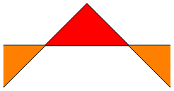
Let us illustrate the effects of some of these methods on the following example.



copy \begin{tikzpicture} \draw [red] (0,0) -- (1,1) -- (2,0); \draw [blue] (0,0.5) -- (2,0.5); \end{tikzpicture}

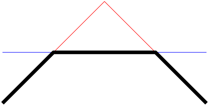
We have two lines, both start on the left-hand-side. Our goal is to get a new path consisting of the intersections segments on the lower part of the picture, i.e. we would like to see



copy \begin{tikzpicture} % this is our goal -- but computed automatically. \draw [black] (0,0) -- (0.5,0.5) -- (1.5,0.5) -- (2,0); \end{tikzpicture}

In order to let fillbetween compute the target path, we assign names to the input paths, compute the intersections – and recombined them using \pgfcomputeintersectionsegments.

Attention:

Before you want to replicate this example, you may want to read about intersection segments which is a much simpler way to get the same effect!

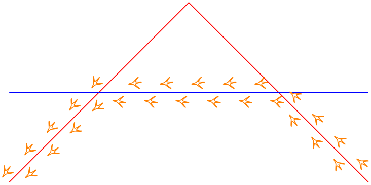
Note that this operates on a relatively low level. However, you can easily insert these statements into a \pgfextra in order to embed it into TikZ. This allows access to any TikZ options, including decorate:

Attention:

Before you want to replicate this example, you may want to read about intersection segments which is a much simpler way to get the same effect!

\pgfgetintersectionsegmentpath{1 or 2}{index} ¶

Defines \pgfretval to contain the desired path segment as softpath.

The result has the same quality as a path returned by \pgfgetpath and can be used by means of \pgfsetpath, \pgfsetpathandBB, or \pgfaddpathandBB.

The value 1 or 2 resembles the argument of a preceding call to \pgfcomputeintersectionsegments: it identifies which of the two paths for which intersections have been computed is to be selected.

The second argument index is a number \(0 \le i < N\) where \(N\) is the total number of computed segments. The total number of computed segments is returned by \pgfcomputeintersectionsegments.

This macro is part of fillbetween.

\tikzgetnamedpath{string name} ¶

Defines \pgfretval to contain the softpath associated with string name. The string name is supposed to be the value of name path or name path global.

The resulting value is a softpath, i.e. it has the same quality as those returned by \pgfgetpath.

This macro is part of fillbetween.

\tikznamecurrentpath{string name} ¶

Takes the current softpath (the one assembled by previous moveto, lineto, or whatever operations), and assigns the name string name to it.

This macro is part of fillbetween.

\pgfcomputereversepath{\softpathmacro} ¶

Takes a softpath \softpathmacro and computes its reversed path.

It stores the resulting softpath into \pgfretval.

This macro is part of fillbetween.

\pgfgetpath{\softpathmacro} ¶

Stores the current softpath into the macro \softpathmacro.

See also \tikzgetnamedpath.

This macro is part of pgf.

\pgfsetpath{\softpathmacro} ¶

Replaces the current softpath from the macro \softpathmacro.

This does not update any bounding boxes. Note that this takes a softpath as it is, no transformation will be applied. The only way to modify the path and its coordinates is a decoration or a canvas transformation.

This macro is part of pgf.

\pgfaddpath{\softpathmacro} ¶

Appends the softpath from the macro \softpathmacro to the current softpath.

This does not update any bounding boxes. Note that this takes a softpath as it is, no transformation will be applied. The only way to modify the path and its coordinates is a decoration or a canvas transformation.

This macro is part of pgf.

\pgfsetpathandBB{\softpathmacro} ¶

Replaces the current softpath from the macro \softpathmacro.

This updates the picture’s bounding box by the coordinates found inside of \softpathmacro. Aside from that, the same restrictions as for \pgfsetpath hold here as well.

This macro is part of fillbetween.

\pgfaddpathandBB{\softpathmacro} ¶

Appends the softpath of macro \softpathmacro to the current softpath.

This updates the picture’s bounding box by the coordinates found inside of \softpathmacro. Aside from that, the same restrictions as for \pgfsetpath hold here as well.

This macro is part of fillbetween.

\pgfpathreplacefirstmoveto{\softpathmacro} ¶

Takes a macro containing a softpath on input, replaces its first moveto operation by a lineto operation and returns it as \pgfretval.

The argument \softpathmacro is one which can be retrieved by \pgfgetpath.

This macro is part of fillbetween.

\pgfintersectionofpaths{first}{second} ¶

The pgf basic layer command to compute intersections of two softpaths. In contrast to the name path method provided by TikZ, this command accepts different argument: first and second are supposed to set paths, i.e. they should contain something like \pgfsetpath{\somesoftpath}.

Results are stored into variables of the current scope.

This macro is part of pgf.

\tikzpathintersectionsegments[options with prefix /tikz/segments] ¶

An alias for \tikzset{intersection segments={options}}.

\pgfpathcomputesoftclippath{\inputsoftpath}{\softclippath} ¶

Does the work for soft clip: it computes the soft-clip path of \inputsoftpath when it is clipped against \softclippath.

The algorithm has been tested and written for rectangular soft clip paths. It will accept complicated clip paths, and might succeed with some of them. Nevertheless, rectangular soft clip paths are the ones which are supported officially.

See soft clip for details.