Manual for Package pgfplots
2D/3D Plots in LATeX, Version 1.18.2
https://github.com/pgf-tikz/pgfplots
Utilities and Basic Level Commands
9.4Specifying Basic Coordinates
-
\pgfplotspointaxisxy{
 x coordinate
 }{y coordinate}
}{y coordinate}
-
\pgfplotspointaxisxyz{
x coordinate}{y coordinate}{z coordinate}
Point commands like \pgfpointxy which take logical, absolute coordinates and return a low-level point. Every transformation from user transformations to logarithms is applied.
Since the transformations are initialized after the axis is complete, this command needs to be postponed (see \pgfplotsextra).
This command is the basic level variant of axis cs:x coordinate,y coordinate,z coordinate.
Note that this is also the default coordinate system during the visualization phase; in other words: if you write \draw (1,2) -- (1,4), pgfplots will automatically use (axis cs:1,2) -- (axis cs:1,4).
-
\pgfplotspointaxisdirectionxy{
x coordinate}{y coordinate}
-
\pgfplotspointaxisdirectionxyz{
x coordinate}{y coordinate}{z coordinate}
Point commands like \pgfpointxy which take logical, relative coordinates and return a low-level point. Every transformation from user transformations to logarithms is applied. The difference to \pgfplotspointaxisxy is that the shift of the linear transformation is skipped here (compare disabledatascaling).
This command is the basic level variant of axis direction cs:x coordinate,y coordinate,z coordinate. Please refer to the documentation of
axis direction cs for more details.
Use this command whenever something of relative character like directions or lengths need to be supplied. One use case is to draw ellipses:
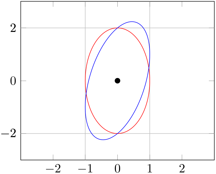
% Preamble: \pgfplotsset{width=7cm,compat=1.18}
\begin{tikzpicture}
\begin{axis}[
xmin=-3, xmax=3,
ymin=-3, ymax=3,
extra x ticks={-1,1},
extra y ticks={-2,2},
extra tick style={grid=major},
]
\draw [red] \pgfextra{
\pgfpathellipse{\pgfplotspointaxisxy{0}{0}}
{\pgfplotspointaxisdirectionxy{1}{0}}
{\pgfplotspointaxisdirectionxy{0}{2}}
% see also the documentation of
% 'axis direction cs' which
% allows a simpler way to draw this ellipse
};
\draw [blue] \pgfextra{
\pgfpathellipse{\pgfplotspointaxisxy{0}{0}}
{\pgfplotspointaxisdirectionxy{1}{1}}
{\pgfplotspointaxisdirectionxy{0}{2}}
};
\addplot [only marks,mark=*] coordinates
{ (0,0) };
\end{axis}
\end{tikzpicture}
Since the transformations are initialized after the axis is complete, this command needs to be provided either inside of a TikZ \path command (like \draw in the example above) or inside of \pgfplotsextra.
-
\pgfplotspointrelaxisxy{
rel x coordinate}{rel y coordinate}
-
\pgfplotspointrelaxisxyz{
rel x coordinate}{rel y coordinate}{rel z coordinate}
Point commands which take relative coordinates such that \(x=0\) is the lower \(x\)-axis limit and \(x=1\) the upper \(x\)-axis limit.
These commands are used for rel axis cs.
Please note that the transformations are only initialised if the axis is complete! This means you need to provide \pgfplotsextra.
-
\pgfplotspointdescriptionxy{
\(x\) fraction}{\(y\) fraction}
-
\pgfplotsqpointdescriptionxy{
\(x\) fraction}{\(y\) fraction}
Point commands such that {0}{0} is the lower left corner of the axis’ bounding box and {1}{1} the upper right one; everything else is in between. The ‘q’ variant is quicker as it doesn’t invoke the math parser on its arguments.
They are used for axis description cs, see Section 4.9.1.
-
\pgfplotspointaxisorigin 
A point coordinate at the origin, \((0,0,0)\). If the origin is not part of the axis limits, the nearest point on the boundary is returned instead.
This is the same coordinate as returned by the origin anchor.
-
\pgfplotstransformcoordinatex{
x coordinate of an axis}
-
\pgfplotstransformcoordinatey{
y coordinate of an axis}
-
\pgfplotstransformcoordinatez{
z coordinate of an axis}
Defines \pgfmathresult to be the low-level pgf coordinate corresponding to the input argument.
The command applies any [xyz] coord trafo keys, data scalings and/or logarithms or whatever pgfplots does to map input coordinates to internal coordinates.
The result can be used inside of a \pgfpointxy statement (i.e. it still needs to be scaled with the respective pgf unit vector).
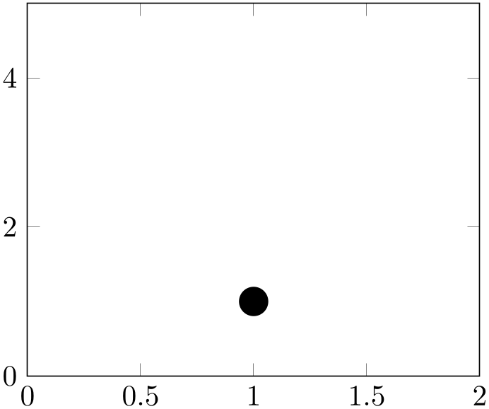
% Preamble: \pgfplotsset{width=7cm,compat=1.18}
\begin{tikzpicture}
\pgfplotsset{compat/pgfpoint substitution=1.3}
\begin{axis}[xmin=0,xmax=2,ymin=0,ymax=5]
\pgfplotsextra{
\pgfplotstransformcoordinatex{1}
\let\xcoord=\pgfmathresult
\pgfplotstransformcoordinatey{1}
\let\ycoord=\pgfmathresult
\pgfpathcircle
{\pgfqpointxy{\xcoord}{\ycoord}}
{5pt}
\pgfusepath{fill}
}
\end{axis}
\end{tikzpicture}
Note that pgfplots substitutes \pgfqpointxy by \pgfplotspointaxisxyz by default – and this command implicitly transforms coordinates anyway. In order to see the difference, the preceding example first disables this automatic substitution of coordinate systems by means of compat/pgfpoint substitution=1.3. The result of this command is also available as math method transformcoordinatex (see the documentation for axis cs).
Please note that the transformations are only initialised if the axis is complete. This means you need to provide \pgfplotsextra as is shown in the example above.
-
\pgfplotstransformdirectionx{
x direction of an axis}
-
\pgfplotstransformdirectiony{
y direction of an axis}
-
\pgfplotstransformdirectionz{
z direction of an axis}
Defines \pgfmathresult to be a low-level pgf direction vector component.
A direction vector needs to be added to some coordinate in order to get a coordinate, compare the documentation for \pgfplotspointaxisdirectionxy and axis direction cs.
The argument
x direction of an axis
is processed in (almost) the same way as for the macro which operates on absolute positions,
\pgfplotstransformcoordinatex. The only difference is that directions need no shifting transformation.
The result of this command is also available as math method transformdirectionx (see the documentation for axis direction cs).
See axis direction cs for details and examples about this command.
-
\pgfplotspointunitx 
-
\pgfplotspointunity 
-
\pgfplotspointunitz 
Low-level point commands which return the canvas \(x\), \(y\) or \(z\) unit vectors.
The \pgfplotspointunitx is the pgf unit vector in \(x\) direction.
These vectors are essentially the same as \pgfqpointxyz{1}{0}{0}, \pgfqpointxyz{0}{1}{0}, and \pgfqpointxyz{0}{0}{1}, respectively.
The unit \(z\) vector is only defined for three dimensional axes.
-
\pgfplotsunitxlength 
-
\pgfplotsunitylength 
-
\pgfplotsunitzlength 
-
\pgfplotsunitxinvlength 
-
\pgfplotsunityinvlength 
-
\pgfplotsunitzinvlength 
Macros which expand to the vector length \(\lVert x_i \rVert \) of the respective unit vector \(x_i\) or the inverse vector length, \(1/\lVert x_i \rVert \). These macros can be used inside of \pgfmathparse, for example.
The \(x_i\) are the \pgfplotspointunitx variants.
-
\pgfplotsqpointoutsideofaxis{
three-char-string}{coordinate}{normal distance}
Provides a point coordinate on one of the available four axes in case of a two dimensional figure or on one of the available twelve axes in case of a three dimensional figure.
The desired axis is uniquely identified by a three character string, provided as first argument to the command. The first of the three characters is ‘0’ if the \(x\)-coordinate of the specified axis passes through the lower axis limit. It is ‘1’, if the \(x\)-coordinate of the specified axis passes through the upper axis limit. Furthermore, it is ‘2’ if it passes through the origin. The second character is also either 0, 1 or 2 and it characterizes the position on the \(y\)-axis. The third character is for the third dimension, the \(z\)-axis. It should be left at ‘0’ for two dimensional plots. However, one of the three characters should be ‘v’, meaning the axis varies. For example, v01 denotes \(\{ (x,y_{\min },z_{\max }) \vert x \in \mathbb {R} \}\).
The second argument,
coordinate
is the logical coordinate on that axis. Since two coordinates of the axis are fixed,
coordinate
refers to the varying component of the axis. It must be a number without unit; no math
expressions are supported here.
The third argument
normal distance
is a dimension like 10pt. It shifts the coordinate away from the designated axis in direction of the outer normal
vector. The outer normal vector always points away from the axis. It is computed using
\pgfplotspointouternormalvectorofaxis.
There are several variants of this command which are documented in the source code. One of them is particularly useful:
-
\pgfplotsqpointoutsideofaxisrel{
three-char-string}{axis fraction}{normal distance}
This point coordinate is a variant of
\pgfplotsqpointoutsideofaxis which
allows to provide an
axis fraction
instead of an absolute coordinate. The fraction is a number between \(0\) (lower axis limit) and \(1\) (upper axis limit),
i.e. it is given in percent of the total axis. It is possible to provide negative values or values larger than one.
The \pgfplotsqpointoutsideofaxisrel command is similar in spirit to rel axis cs.
There is one speciality in conjunction with reversed axes: if the axis has been reversed by x dir=reverse and, in addition, allow reversal of rel axis cs is true, the value \(0\) denotes the upper limit while \(1\) denotes the lower limit. The effect is that coordinates won’t change just because of axis reversal.
-
\pgfplotspointouternormalvectorofaxis{
three-char-string}
A point command which yields the outer normal vector of the respective axis. The normal vector has length \(1\) (computed with \pgfpointnormalised). It is the same normal vector used inside of \pgfplotsqpointoutsideofaxis and its variants.
The output of this command will be cached and reused during the lifetime of an axis.
-
\pgfplotsticklabelaxisspec{
x, y or z}
Expands to the three character identification for the axis containing
tick labels for the chosen axis, either
x,
y
or
z.
-
\pgfplotsvalueoflargesttickdimen{
x, y or z}
Expands to the largest distance of a tick position to its tick label bounding box in direction of the outer unit normal vector. It does also include the value of the ticklabel shift key.
This value is used for ticklabel cs.
-
\pgfplotsmathfloatviewdepthxyz{
x}{y}{z}
-
\pgfplotsmathviewdepthxyz{
x}{y}{z}
Both macros define \pgfmathresult to be the “depth” of a three dimensional point \(\bar x = (x,y,z)\). The depth is defined to be the scalar product of \(\bar x\) with \(\vec d\), the view direction of the current axis.
For \pgfplotsmathfloatviewdepthxyz, the arguments are parsed as floating point numbers and the result is encoded in floating point. A fixed point representation can be generated with \pgfmathfloattofixed{\pgfmathresult}.
For \pgfplotsmathviewdepthxyz, TeX arithmetics is employed for the inner product and the result is assigned in fixed point. This is slightly faster, but has considerably smaller data range.
Both commands can only be used inside of a three dimensional pgfplots axis (as soon as the axis is initialised, see \pgfplotsextra).
-
\ifpgfplotsthreedim
true code\elseelse code\fi
A
TeX
\if which evaluates the
true code
if the axis is three dimensional and the
else code
if not.