Manual for Package pgfplots
2D/3D Plots in LATeX, Version 1.18.2
https://github.com/pgf-tikz/pgfplots
Utilities and Basic Level Commands
9.6Accessing Point Coordinate Values
During the visualization phase, pgfplots provides access to the currently processed coordinate and its values.
This access requires a call to specific macros. These macros write the coordinate values to some publicly available key–value pairs. Then, the current point’s \(x\), \(y\), \(z\), and color data can be accessed.
-
\pgfplotspointgetcoordinates 
-
\pgfplotspointgetcoordinates{
 point
point }
}
-
1. Without arguments. In this case, it returns values of the point which is about to be processed by the current plot handler.
-
2. With an argument in curly braces. In this case, it expects a coordinate and assigns the keys accordingly. Note that this command merely supports two-dimensional axes and assigns only /data point/x and /data point/y.
After invoking the macro, the following keys will be set:
/data point/x will contain the current point’s \(x\)-coordinate.
/data point/y will contain the current point’s \(y\)-coordinate.
/data point/z will contain the current point’s \(z\)-coordinate (if applicable).
/data point/meta will contain the current point’s point meta value (if applicable).
/data point/index will contain the current point’s index in the coordinate stream. This is actually the same as \coordindex.
This command actually supports two modes of operation:
The returned values are the same as they can be read on the axes, they are also the same as you would write them into axis cs.
This means that any x coord inv trafo has been applied on the value. It also means that the exponential function has been called even though the internal coordinate was present in log format.
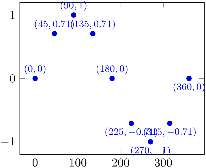
This function is implicitly called for any scatter plot (including nodes near coords). This allows to access all coordinate values at once:

% Preamble: \pgfplotsset{width=7cm,compat=1.18}
\begin{tikzpicture}
\begin{axis}
\addplot+ [
domain=0:360,
samples=9,
only marks,
nodes near coords={%
\footnotesize
$(\pgfmathprintnumber
{\pgfkeysvalueof{/data point/x}},
\pgfmathprintnumber
{\pgfkeysvalueof{/data point/y}})$%
},
] {sin(x)};
\end{axis}
\end{tikzpicture}
The example works because \pgfplotspointgetcoordinates is part of the standard implementation of nodes near coords; the resulting values are directly available. Note that the preceding example would have been simpler if we would have printed just one value: nodes near coords resorts to the point meta. And that, in turn, contains the \(y\)-coordinate anyway by default.
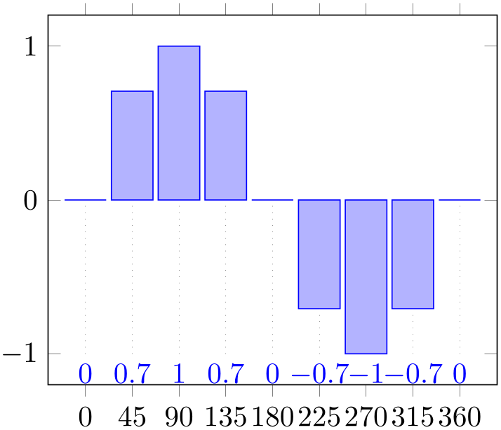
A more advanced example would be a ybar plot in which nodes shall be placed at the lower end of the axis, together with some dotted lines to the respective bars:

% Preamble: \pgfplotsset{width=7cm,compat=1.18}
\begin{tikzpicture}
\begin{axis}[
ybar,
nodes near coords,
%
% we want to provide absolute 'at' values
% for the nodes:
scatter/position=absolute,
every node near coord/.style={
at={(\pgfkeysvalueof{/data point/x},-1)},
% pretty printing:
anchor=north,
/pgf/number format/fixed,
/pgf/number format/precision=1,
% assign a name which can be referenced below:
name=NNC\pgfkeysvalueof{/data point/index},
},
% ... draw a dotted line between
% the marker and the bar:
/pgfplots/scatter/@post marker code/.add code={}{
\draw [dotted,help lines]
                                (NNC\pgfkeysvalueof{/data
                    point/index})
                                --
                    (\pgfkeysvalueof{/data point/x},
{min(0,\pgfkeysvalueof{/data point/y})});
},
% assign suitable tick labels:
xtick=data,
]
% some dummy data:
\addplot+ [
domain=0:360,
bar width=360/9,
samples=9,
] {sin(x)};
\end{axis}
\end{tikzpicture}
Again, the command is used implicitly as part of nodes near coords and does not occur in the example as such.
See also the related example online under https://tex.stackexchange.com/a/141006. It demonstrates how to place the nodes generated by nodes near coords based on the value (either inside of a bar or above it).
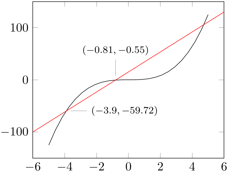
The following example uses an argument in curly braces for which we seek coordinate values:

% Preamble: \pgfplotsset{width=7cm,compat=1.18}
% requires \usetikzlibrary{intersections}
\begin{tikzpicture}
\begin{axis}
\addplot [name path=A] {x^3};
\draw [red,name path=HelperLine]
(axis cs:-6,-100) -- (axis cs:6,130);
\draw [
font=\footnotesize,
name intersections={of=A and HelperLine},
]
node [pin={right:
\pgfplotspointgetcoordinates{(intersection-1)}
$(\pgfmathprintnumber[fixed]{
\pgfkeysvalueof{/data point/x}},
\pgfmathprintnumber[fixed]{
\pgfkeysvalueof{/data point/y}})$
}
] at (intersection-1) {}
node [pin={
\pgfplotspointgetcoordinates{(intersection-2)}
$(\pgfmathprintnumber[fixed]{
\pgfkeysvalueof{/data point/x}},
\pgfmathprintnumber[fixed]{
\pgfkeysvalueof{/data point/y}})$
}
] at (intersection-2) {};
\end{axis}
\end{tikzpicture}
The example computes and names intersections of A and HelperLine. The following code generates pins at
the intersections. To this end, it uses
\pgfplotspointgetcoordinates{ point
point } which defines /data point/x and
/data point/y. These values are then formatted using
\pgfmathprintnumber.
In its second mode,
\pgfplotspointgetcoordinates{ point
point } expects one of two things as
 point
point :
:
-
1. a basic-level pgf point like \pgfpointanchor{A}{center} or
-
2. a TikZ point like (A.base) or (3,5).
-
\pgfplotspointgetnormalizedcoordinates 
A macro which is very similar to \pgfplotspointgetcoordinates. Consequently, it is also supposed to be called during the visualization phase.
It assigns the very same output macros, but the values are different. More precisely, it defines the macros
/data point/x will contain the current point’s normalized \(x\)-coordinate.
/data point/y will contain the current point’s normalized \(y\)-coordinate.
/data point/z will contain the current point’s normalized \(z\)-coordinate (if applicable).
/data point/meta will contain the current point’s point meta value (if applicable).
/data point/index will contain the current point’s index in the coordinate stream. This is actually the same as \coordindex.
The keyword normalized means that the values are in a suitable numerical form which can be consumed by the axis. To be more specific: any user x coord inv trafo is ignored. An important example would be symbolic x coords: the normalized coordinates would be some associated numbers, not the symbols. The results returned by \pgfplotspointgetcoordinates would be the symbols. For logarithm axes, the normalized values are the logs.
Typically, normalized values are much more useful when you want to apply some math operation like averaging or subtraction.
This function needs to be called explicitly. It is currently used by ybar stacked to align nodes near coords.